
The Assistant tool provides us with two methods of regression and a response optimizer for multiple regression. As with all the assistant tools, guidance is offered on the setup of the study and on the output. There are less options to choose from but the dialog box is simpler to use.
Here, we will use the Assistant tool to run a fitted line plot and then pick between Linear, Quadratic, and Cubic models for data on Hubble's constant.
Hubble's law describes the relationship between the distance of a galaxy and the velocity at which it is moving away from us. The greater the distance, the greater the velocity of recession. The data comes from observations on recession velocity of Nebula and its distance from the Earth.
The data can be obtained from the Data and Story Library. The following link will take us to the Hubble results:
http://lib.stat.cmu.edu/DASL/Datafiles/Hubble.html
The data can be copied and pasted directly into Minitab.
The following steps will use the Assistant menu to generate a fitted line plot.
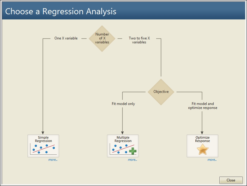
- Go to the Assistant menu and select Simple Regression from the decision tree.
- In Y column:, enter
Recession Velocity. - In X column:, enter
distance. - Ensure that the Choose for me option is selected for the type of regression model and then click on OK.
The assistant regression model will output several graphical report pages. The first page is a report card with many notes or warnings on the analysis. This will check the number of samples in the study and unusual data, and will contain notes about the normality of the residuals.
The second page, that is, the prediction report, contains the fitted regression model and prediction intervals. Also included on this output are prediction intervals for a table of x values and their predicted y values.
Unusual data points are highlighted for values that are more than two standard errors from the predicted values. In this example, the result in row 16 is flagged up as unusually high.
The residual plots will indicate the types of patterns that may indicate problems with the fitted model under the residual plots. By default, only the residuals versus fitted values is generated. If we know that the data is in a time order, then we would tick the option within the dialog box stating that data is in the time order. This would then generate the residuals versus order of the data.
The fourth page, that is, the model selection report, shows the model fitted. It will pick between the Linear, Quadratic and Cubic models by using the R-squared adjusted term. Should we wish to pick a different model to the one fitted we would select the relevant option directly from the dialog box.
The last page, that is, the summary report, presents the results of the regression. The P-value for the study is listed and the null hypothesis is restated as the question "Is there a relationship between Y and X?", which can make interpretation of the P-value easier. When a linear regression model is fitted, the correlation score is also produced. Comments are automatically completed for the data and can be edited.
Strictly speaking, Hubble's law is stated as Recession velocity = H0*Distance, where H0 refers to Hubble's constant. The recession velocity at 0 distance should be 0. Both the fitted line plot and the assistant regression will fit the data for a nonzero intercept. To fit a regression model without an intercept, we would use the Regression or General Regression tools. We can remove the fit for the intercept from the option's subdialog.