There are two tools for fitting trends in Minitab: Trend analysis and double exponential smoothing. Both of these are used to look at the trends in healthcare expenditure in the U.S. The dataset we will look at runs from 1995 to 2011. The values each year are given as a percentage of the GDP and per capita values in dollars.
We will compare the results of a trend analysis plotting a linear trend with double exponential smoothing and produce forecasts for the next three years.
This data was obtained from www.quandl.com.
The following steps will plot the trend and double exponential smoothing results with three years of future forecasts.
- Open the
Healthcare.mtwworksheet. - For the trend analysis, go to the Stat menu, then Time Series option and select Trend Analysis.
- Enter
'Value (%)'in the Variable section. - Check the box for Generate forecasts, and in Number of forecasts, enter
3. - Click on the Time button. Select the radio button for the Stamp section and enter
Yearinto the Stamp section. - Click on OK.
- Click on the Graphs button and select the Four in one residuals option. Click on OK in each dialog box.
- For double exponential smoothing, go back to the Time Series menu and select Double Exp Smoothing.
- Enter
'Value (%)'in the Variable: section. - Follow steps 3 to 6 to stamp the axis with the year and generate residual plots.
Trend analysis can fit trends for Linear, Quadratic, Exponential, and S-Curve models, and works work best when there is a constant trend of the previous types to model in the data. The trend analysis tools use a regression model to fit our data over time.
Double exponential smoothing is best used when the trend varies over time. With the 'Value (%)' data, we should see a change in the trend slope for the period from 2000 to 2003. Because of this, the trend analysis models will not provide an adequate fit to the varying trends in our data.
Double exponential smoothing will use a trend component and a level component to fit to the data. The level is used to fit to the variation around the trend, and the trend is used to fit to the trend line. The fitted line is generated from two exponential formulas. The fitted value at time t is given by the addition of the level and trend components as shown in the following equation:
Here, the level at time t is given as follows:
Also, the trend at time t is given as follows:
Higher values of weight for the level will, therefore, place more emphasis on the most recent results. This makes the double exponential smoothing react more quickly to variations in the data.
Higher trend values will make the trend line react more quickly to changes in the trend; lower values will give a smoother trend line. Lower values for trend will approach the linear trend.
Minitab will calculate the optimal ARIMA weights from an ARIMA (0,2,2) model looking to minimize the sum of squared errors.
For both trend analysis and double exponential smoothing, it is appropriate to check residual plots to verify the assumptions of the analysis.
The accuracy measures in the output form a useful way of comparing the models to each other The measures shown in the output form are as follows:
When comparing different models, the lower these figures, the better the fit to the data.
Here, we should see that double exponential smoothing provides a better fit as we have changes in the trend of the data. We can compare the percentage results to the per capita data and check whether the double exponential or the trend analysis provides a better approach for this new column.
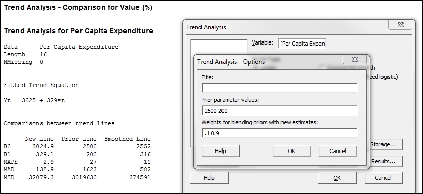
With trend analysis, we can enter historical parameter estimates in options. This will generate a comparison of the new trend and the prior values. The prior and new values can also be blended with each other by specifying a weight for the blending. Parameters and weights must be entered in the order displayed in the trend analysis. If in a previous study, we had obtained a trend of ![]() , then this would be entered into the Prior parameter values section as shown in the following screenshot. The weights for blending each term can be entered as well; these values should be between 0 and 1.
, then this would be entered into the Prior parameter values section as shown in the following screenshot. The weights for blending each term can be entered as well; these values should be between 0 and 1.