
We will use the 1-Sample t-test to investigate the population mean for measures of the economy. The data here is for the UK Gross Domestic Product (GDP). This is often used as a measure of the health of an economy. We will test to see if the percentage growth of GDP per quarter for the UK is equal to zero.
The data for this example was obtained from the Guardian newspaper's website and can be found at http://www.guardian.co.uk/news/datablog/2009/nov/25/gdp-uk-1948-growth-economy.
A direct link to the Google Docs spreadsheet is provided at https://docs.google.com/spreadsheet/ccc?key=0AonYZs4MzlZbcGhOdG0zTG1EWkVPX1k1VWR6LTd1U3c#gid=10.
Enter the results shown in the following screenshot into the worksheet. The UK GDP file1.mtw file is also provided on the Packt Publishing website at http://www.packtpub.com/support.
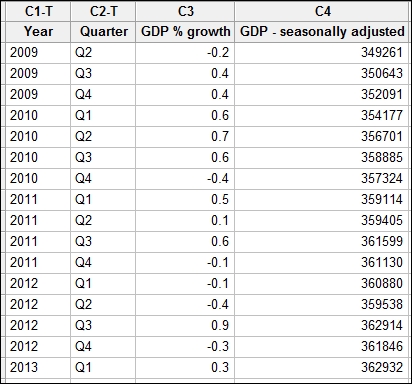
The percentages given in the previous screenshot are rounded figures. To obtain a more precise estimate of the change in percentage, we will calculate this figure. Then, we will run the t-test.
The following example will calculate the percentage change in GDP from the seasonally adjusted data before using a t-test to compare the mean percentage growth to 0:
- Go to the Calc menu, select Calculator…, and enter the expression as shown in the following screenshot:

- Click on OK.
- Go to the Stat menu and then Basic Statistics and select 1-Sample t….
- Enter the %change column into the section for the variables as shown in the following screenshot:
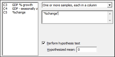
- Check the option for Perform hypothesis test and enter a mean of
0. - Click on the Graphs… button, select Individual value plot, and click on OK twice.
The calculator is used in the first step to find the percentage change using the lag function. The lag(c4,1) function moves the results of column 4 one row down, allowing a comparison of a column with itself one row later.
The null hypothesis of this test is set to a mean of 0 percent. The results come out with a mean of 0.255 percent and a 95 percent confidence interval between 0.017 percent and 0.493 percent. Finally, the P-value for this test is 0.038.
This indicates that the mean %change per quarter is not zero.
The drop-down box above the variables section allows us to choose between using data entered as columns in the worksheet or summarized values of means and standard deviations.
We should check the assumptions of running a t-test. It is random, independent data, and that the population follows a normal distribution, although t-tests are relatively robust to greater than 20 samples that lack normality.
It is useful to run a time series plot to observe variation over time and a normality test.
- The Time series plot recipe in Chapter 2, Tables and Graphs
- The Checking if data follows a normal distribution recipe
- The Finding critical t-statistics using the probability distribution plot recipe