
A balanced ANOVA is one where all combinations of factors have the same number of observed results.
Here, we will look at the analysis of a designed experiment. The study is on an automobile filter to reduce pollution. This study looks at the noise properties of the filter. The response of the noise level is in decibels. The factors include vehicle size—1 2 3, representing small to large, type of filter—1 representing standard and 2 representing octel, and side—1 representing right and 2 representing left.
We will use a balanced ANOVA to study the effect on the results as all treatment conditions have the same number of observations. The terms in the model will be checked for significance using an alpha of 0.05. All main effects and interactions will be included in the model and we will produce residual plots to check the assumptions of using ANOVA.
The data and story behind this example are available from StatLib at http://lib.stat.cmu.edu/DASL/Stories/airpollutionfilters.html.
Copy the data into Minitab and label the columns appropriately.
The filter noise.mtw file is also provided on the Packt Publishing website.
The following steps will run the balanced ANOVA with all the main effects and interactions:
- Navigate to Stat | ANOVA and click on Balanced ANOVA.
- Enter
Noiseinto the Responses field andSize,Type, andSideas Factors. Place the pipe symbol (|) between the factors, as indicated in the following screenshot: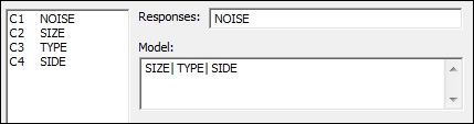
- Click on OK to run the analysis.
- Go to the results in the session window. From the analysis of the variance table, check the terms that are significant. Use a decision of 0.05 for the p-value.
- The three-way interaction term
Size*Type*Sideis significant. The model must be hierarchical, therefore we need to include all the two-way and main effects terms to calculate the model. Use Ctrl + E to return to the last dialog box to select the residual plots. - Click on the Graphs button.
- Click on the radio button for Four in One residuals.
- Click on OK in each dialog.
The balanced ANOVA and general linear model tools can be used with up to 31 factors. The model must be hierarchical; this means that the inclusion of the three-way Size*Type*Side interaction needs to include all the two-way interactions between Size, Type, and Side.
The residual plots can be generated as individual pages or as the Four in one option, as used here. This produces the four residuals on one page as a diagnostic plot. This allows us to check the assumptions of the residual error, which are normally distribution and homoscedasticity.
If we include random factors, these must be entered into the model and then declared as a random factor in the section for Random Factors:. They must be included in both sections for the model to work.
The following information illustrates the use of the notation of pipe, exclamation, and star to specify the model terms. The pipe symbol or exclamation mark can be used as a shortcut to run all interactions between the factors. The |
and ! marks can be used interchangeably.
For example, if we use factors of A, B, and C, then enter the factors as A!B!C into the design, this will specify a model using the A B C AB AC BC ABC terms. If we had just used A!B C, the model would be A B C AB.
Interactions can be entered with the use of a * symbol between factors. Entering A B C A*B B*C will generate a model of A B C AB BC.
Terms can be excluded in a model by the use of a minus sign. By specifying the model as A|B|C – A*B*C, we would have a model of A B C AB AC BC.
The general linear model tool from ANOVA can also be used for balanced designs, one-way ANOVA, two-way ANOVA, and to define nested designs. The only option that balanced designs offer us over the general linear model is the option to run a restricted model. The restricted model can be used when both fixed and random terms are included in the design.