
GLM or General Linear Model is a general tool for ANOVA. As such, we see that it will run studies from factors 1 to 31, and can include nesting or random factors.
For this example, we will look at a larger dataset. The data is for crash test dummies that have been used to look at forces in controlled crash environments. The National Transportation Safety Board collected data from crashing vehicles into a wall at 35 mph. Columns contain information on the make and model of the car. Head injury criterion, chest deceleration, left femur load, right femur load, D/P (whether the dummy was in the driver or passenger seat), protection, doors, year of the car, weight in pounds, and size of the vehicle.
We will look at a few of the factors to study the effect on chest deceleration. It is not possible to investigate all interactions in the data. This is due to some missing values in the results, and not all combinations of levels are possible. We will start by focusing on just a few.
The instructions will reduce the model step-by-step, removing the interactions in the model. Alpha for the decision level is used as 0.05 in this data.
As a note, the recipe is meant to be indicative of how such a study can be run and is not an exclusive study into a full model. We should build on these instructions and use the example as a base for a more in-depth study. We should also be careful of associations as a cause until we can discount other reasons. This data was also used in support of legal arguments over safety.
The crash test data can be found at the following link:
http://lib.stat.cmu.edu/DASL/Datafiles/Crash.html
The results can be copied and pasted directly into Minitab.
The following instructions will specify a model with several interactions and then reduce the design by removing steps highest p-values:
- Navigate to Stat | ANOVA | General Linear Model and click on Fit General Linear Model.
- Enter
'Chest decel'in the Responses: field and enter'D/P'ProtectionDoorsandSizeinto the Factors: field as shown in the following screenshot: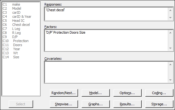
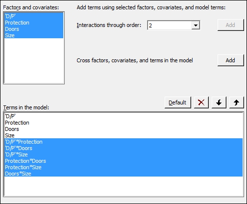
- To enter interactions for the factors, click on the Model… button.
- Highlight the factors within the Factors and covariates: section and click on the Add button next to Interactions through order:, as shown in the following screenshot:
- Click on OK and return to the session window to check the results. Look for interactions with a p-value above the decision level.
- Check for the interaction with the highest p-value. From the results shown in the following screenshot, D/P*Size has the highest p-value. Press Ctrl + E to return to the last dialog box:
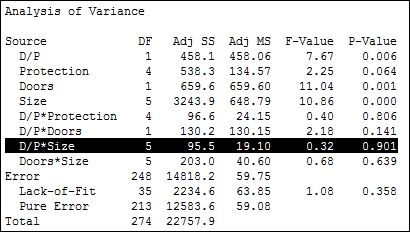
- Click on the Model… button. Then, select the interaction of 'D/P'*Size from the Terms in the model: field and click on the red X to remove this term. Also, remove the terms of Protection*Doors and Protection*Size. These cannot be estimated, as indicated in the session window.
- Return to the session window and look for interactions with a p-value greater than 0.05. As in the previous step, look for the interaction with the highest p-value. Press Ctrl + E to return to the GLM and remove this term from the dialog.
- Repeat steps 6 and 7 until only the interactions with p-values below 0.05 remain in the model.
- Steps 6 and 7 should then be repeated for the main effects, removing each term one by one. Main effects must be included, which are part of an interaction or have a p-value less than 0.05.
- When only the significant terms are left in the model, return to the Fit General Linear Model dialog box and run residual plots. Click on the Graphs button and select the Four in one residuals.
- Click on OK in each dialog box.
- To create main effects plots, navigate to Stat | ANOVA | General Linear Model and click on Factorial Plots.
- The Response: field of
Chest decelshould already have been included and to create charts of the terms included in the model, click on OK.
The data has several missing values in different columns and is unbalanced due to incomplete cells of the study having the same number of results. For example, there are 59 results with two-door vehicles and 84 results with four-door vehicles. The number of doors for vans and pickup trucks are not recorded and are shown as missing. We should be careful of these missing results as they will be left out of the model.
Using the descriptive statistics tables under the Tables menu, we can show the number of observations for each level within each factor. Entering Protection and Size columns in this tool would show us that the driver and passenger airbags are present only in the size group hev, and driver airbags are not present in mini, mpv, pu, and van. This prevents us from looking at interactions between Protection and Size.
As the design is not balanced, the values of the sequential sum of squares and the adjusted sum of squares will be different. The order of the data in the results could change the estimation of the sequential sum of squares. By default, the adjusted sums of squares are used to calculate the significance of the terms. The button for options allows us to change the calculations to use the sequential sum of squares, if required.
We reduce the model one term at a time, starting with the highest order interactions due to the design being unbalanced. At each step, we look for the term with the highest p-value and remove that term. When all two-way interactions are removed or we are left with interactions that are significant, we move to reducing main effects in the same manner. Main effects must still be included even if they are not significant when they are used in an interaction.
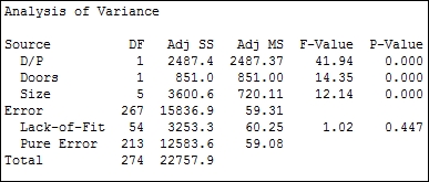
The final model that we should reduce down to when using a p-value of 0.05 as a decision is D/P (Doors and Size), as shown in the following screenshot:
Differences between the levels can be investigated with the use of the comparisons tool in GLM. Pairwise comparisons, or comparisons versus control can be selected. In Minitab v16, this is found within the GLM dialog box.
In Minitab v17, this is accessed from the General Linear Model menu and is available after we have fitted a model.
The results here have only investigated the effects of the factors. The weight of the vehicle will be found as significant when entered as a covariate. In Minitab v17, to identify a covariate, this is added into the Covariates: section of the general linear model dialog box. Interactions with covariates, quadratic or cubic terms for the covariates can be included from the Model section of the General Linear Model dialog box.
The worksheet can be subset to focus on a few results rather than the total. This is useful when a level for a factor is creating a lot of missing cells in the design. For example, removing the vans and pickup trucks from the dataset will mean that we can look at the interaction for Doors*Size for the size of vehicles that we have left in the worksheet.
We should check the residual plots after the study has focused on the significant terms. This is to verify the assumptions of using the analysis of variance on the final model. In this example, a couple of results appear to have high residuals. See the graph in the following screenshot:
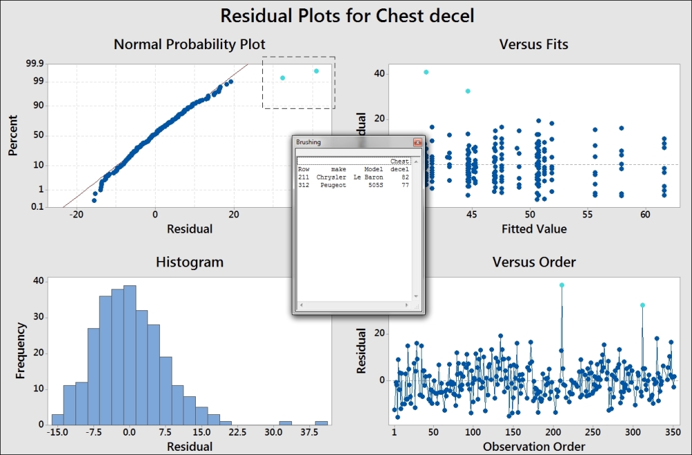
This graph uses the brushing tool to highlight the high values on the probability plot. Its make and model is included to identify the cars associated with these results.
To use the brushing tool, right-click on the chart and select brush from the right-click menu. Highlight the two high residual points by dragging a box around them. Right-click on the graph again and click on Set ID Variables. Enter the make and model columns into the brushing variables to add this information into the Brushing box.
The residuals for the chest deceleration appear to show a slight right-hand skew. The assumptions to run an analysis of variance are that the residuals are distributed normally. For an underlying distribution that is expected to not be distributed normally, the response can be transformed. A lognormal transformation of the results can be used in some cases. The calculator tool in the Calc menu can be used to find the lognormal transformation of chest deceleration. The function is Ln(column) and can be found in the function list of the calculator.
You should take care with transformation of the data to ensure that the reasons for transformation are justified and a logical explanation exists for the shape of the data. Note that in this recipe, using a lognormal transformation of the chest deceleration force will result in residuals that appear more normally distributed. The resultant model from the lognormal results will not be appreciably better than using the untransformed data.
The residuals are produced as regular by default and there are options for standardized or deleted residuals as well.