7.9.  COMPENSATION AND DESIGN USING THE ROOT-LOCUS METHOD

The root-locus technique has been developed previously in Sections 6.14–6.16, and digital computer programs for obtaining the root locus were presented in Section 6.17 (MATLAB) and 6.18. It is a very helpful tool that the control engineer can use in order to study the variation of gain, system parameters, and effect of compensation. We demonstrated in Section 6.14 the migration of poles in the complex plane as the gain of the system was varied from zero to infinity. We obtained the root locus for several feedback systems including the following:

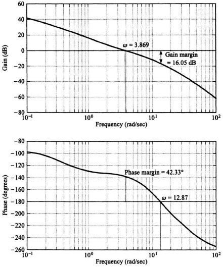
Figure 7.36   Bode diagram for the compensated system of Figure 6.49, where

This was illustrated in Figure 6.60. An analysis of the root locus for this system indicated that it was always unstable, because at least one of the roots of the characteristic equation always occurred in the right-half-plane. This section demonstrates how this system may be compensated by means of a phase-lead network, and/or rate feedback in parallel with position feedback. This problem is followed by considering phase-lag-network compensation for the system illustrated in Figure 6.57. In addition, we shall demonstrate how the control engineer may determine the transient response of the compensated systems in order to meet certain specifications.

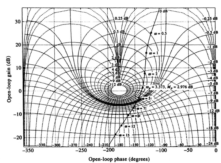
Figure 7.37   Compensation of the system shown in Figure 6.49 for M = 2.976 dB (1.4).

A.  Example of Phase-Lead Network and Rate-Feedback Compensation

Let us attempt to stabilize the system of Figure 6.60 by means of a phase-lead network in cascade with the forward-loop transfer function. The form of its transfer function is given by

We assume that the effect of the pole introduced by the phase-lead network has a negligible effect compared with its zero. Therefore, we assume that the transfer function of the cascaded phase-lead network can be approximated by the zero term only, which is also equivalent to the pure zero obtained with rate feedback in parallel with position feedback (see Figure 7.14a):

The resulting value of G_c(s)G(s)H(s), which is to be examined on the root locus, is given by

We wish to investigate the effect on stability of a variation in α as follows:

Case A :  α = 0.5     Case D :  α = 4
Case B :  α = 1        Case E :  α = 6.
Case C :  α = 2

The resulting root loci for all these cases are presented next. It is important to emphasize at this point that, although we make use of most of the anlaytic tools developed in Section 6.14, we do not use all of them, This omission is due to the fact that some of the analytic techniques developed are too complex to use for higher-order systems. For example, it is very tedious to determine the value of the gain K along the root loci utilizing the relationship given by Eq. (6.133). Fortunately, this can be obtained much more easily with the digital computer program presented in Section 6.18 or by using MATLAB (Section 6.17). The approach taken in presenting the resulting root loci for this problem is to outline the results of the 12 rules developed previously in Section 6.14, and use the digital computer programs of Section 6.18 or by using MATLAB (Section 6.17) wherever it is helpful. In addition, the values of gain obtained using the digital computer program or MATLAB which are pertinent for an intelligent evaluation of the problem will be indicated. It is my feeling that this dual approach is the best procedure to use when explaining the root-locus method.

Case A. α = 0.5. See Figure 7.38 for the root-locus sketch.

Rule 1.  There are four separate loci because the characteristic equation,

1 + G_c(s)G(s)H(s) = 0,

is a fourth-order equation.

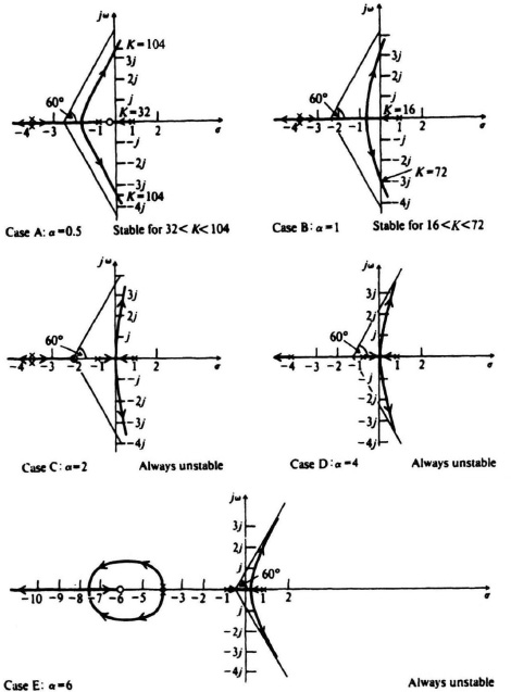
Figure 7.38   Compensation of the root locus shown in Figure 6.60 using a pure zero term where G_c(s) = (s + α).

Rule 2.  The root locus starts (K = 0) from the poles located at 1, −1, and a double pole at −4. One branch terminates (K = ∞) at the zero located at α = −0.5 and three branches terminate at zeros located at infinity.

Rule 3.  Complex portions of the root locus occur in complex-conjugate pairs.

Rule 4.  The portions of the real axis between 1 to −α, −1 to −4, and −4 to ∞ are part of the root locus.

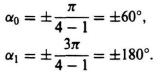
Rule 5.  The branches approach infinity as K becomes large at angles given by

and

Rule 6.  The intersection of the asymptotic lines and the real axis occur at

Rule 7.  Using MATLAB, we found the point of breakaway from the real axis to occur at −1.7549.

Rule 8.  Using MATLAB, we found the intersection of the root locus and the imaginary axis to occur at s = ± j3.3, where the gain is 104, and at the origin, where the gain is 32.

Rule 9.  This rule does not apply here.

Rule 10.  This rule shows that as certain of the loci turn to the right, others turn to the left to ensure that the sum of the roots is a constant.

Rule 11.  This rule does not apply here.

Rule 12.  The root locus does not cross itself.

The resulting root locus indicates that the system is stable when 32 < K < 104.

Case B.  α = 1. See Figure 7.38 for the root-locus sketch. A zero at s = −1 cancels the pole at −1. The resulting root-locus sketch indicates that this system is stable when 16 < K < 72. (The point of breakaway occurs at −0.667.)

Case C.  α = 2. See Figure 7.38 for the root-locus sketch. The resulting root-locus sketch indicates that the system is always unstable, because at least one of the roots of the characteristic equation always occurs in the right half-plane except for the condition where two poles exist at the origin. (The point of breakaway occurs at the origin.)

Case D.  α = 4. See Figure 7.38 for the root-locus sketch. A zero at α = 4 cancels one of the poles located at −4. the resulting root-locus sketch indicates that the system is always unstable since at least one of the roots of the characteristic equation always occurs in the right half-plane. (The point of breakaway occurs at 0.1196.)

Case E.  α = 6. See Figure 7.38 for the root-locus sketch. The resulting root-locus sketch indicates that the system is always unstable, because at least one of the roots of the characteristic equation always occurs in the right half-plane. (The Points of breakway occur at 0.1156 and −4, and a break-in occurs at −7.0611.)

Conclusions of Cases A through E

Interpretation of Figure 7.38 is quite interesting and revealing. It indicates that the exact location of the zero is very important from a stability viewpoint. Cases A and B were the only configurations which had regions of stability. As a matter of fact, the closer the zero lies to the imaginary axis, the greater is its stabilizing effect. This point is very important. Because Case A resulted in larger values of gain, it would result in a more accurate system and is, therefore, preferred to Case B.

The reader should not get the impression that α could be made extremely small (e.g. 0.0001) to satisfy this guideline because you will be paying a penalty in the size of the capacitors and resistors used in a passive phase-lead network. Remember that the form of the zero is (s + α), which can be modified to α[(1/α)s + 1], where 1/α is the time constant of the zero term. Therefore, very small values of α mean that the values of the components (resistors and capacitors) would be too large which is undesirable from a practical viewpoint. If the zero term (s + α) is obtained using rate feedback in cascade with position feedback, as in Figure 7.14a, then you would have to make 1/α = b and very small values of α would mean extremely large values of b. This would require an amplifier in cascade with the rate-feedback sensor (e.g., tachometer or rate gyro), which is undesirable due to the added cost and possible noise problems.

B.  Determination of the Transient Response

The transient response of the system can also be obtained by reasoning along these lines: The transient performance is often dominated by the pair of complex conjugate poles located closest to the origin. This occurs when the other poles are far to the left of the dominant poles, or the other poles are near a zero. The resulting transient components due to these other poles are small under these conditions and diminish rapidly. For this case, the poles closest to the origin are conventionally referred to as the dominant poles. The relative dominance of the closed-loop poles is found from the ratio of the real parts of the complex-conjugate poles. As a general guideline, reasonable dominance exists if the ratios of the real parts are at least five, and there are no zeros nearby. For such conditions, the closed-loop complex-conjugate poles closest to the origin will dominate the transient response. From the discussion of Section 4.2, the expression associated with these complex poles can be given by the following expression [see Eq. (4.3)]:

where ζ = damping ratio, and ω_n = undamped natural frequency. We found in Section 4.2 that the transient response to a unit step input, for ζ < 1, is given by the following expression [see Eq. (4.24)]:

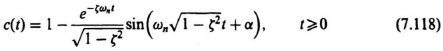
where

α = cos⁻¹(ζ).

Figure 4.3 illustrated the complex-plane location of these dominant poles. The values derived for the time to the first peak [see Eq. (4.29)] and maximum percent overshoot [see Eq. (4.33)] are specifically for a second-order system whose closed-loop transfer function is given by Eq. (7.117). These quantities change if other closed-loop poles and zeros exist in addition to the dominant complex pair. However, if the ratios of the real parts of the various complex-conjugate poles are greater than five and there are no zeros nearby, then the approximation gives reasonable results. The damping ratio determined in this case using the pair of complex-conjugate roots closest to the imaginary axis is defined as the relative damping ratio of the control system.

Expressions for time to the first peak and percent overshoot, which consider other poles and zeros and give more accurate results, can be derived [6]. These expressions assume that

(a)  Other poles are far to the left of the dominant poles, so that the amplitude of transients due to these other poles is small.

(b)  Poles which are not far to the left of the dominant poles are near a zero so that the transient amplitude due to such poles is small.

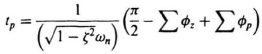
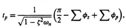
The expressions, for unity-feedback systems, are given by

where

  = sum of the angles from the zeros of C/R to one of the dominant poles,
  = sum of the angles from the zeros of C/R to one of the dominant poles,

and the maximum percent overshoot

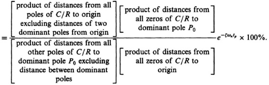
The expression for maximum percent overshoot can be stated symbolically as

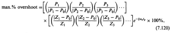
where the first set of brackets represents the product of the ratios of the values of s at which poles occur to their absolute distances from the dominant pole. The second set of brackets represents the product of the ratios of the absolute distances of the zeros from the dominant pole and the values of s at which the zeros occur. Let us next apply these expressions in the following design problem.

C.  Example of Phase-Lag-Network Compensation and Overall System Performance

The concluding design problem we consider using the root locus consists of employing cascaded phase-lag compensation in order to improve the steady-state performance of a feedback control system. The object is to increase its gain while maintaining a good dynamic response. Specifically, we consider the system whose root locus was illustrated in Figure 6.57. For this system

The root locus of Figure 6.57 indicated that the system was stable when 0 < K < 180. Let us assume that a damping factor of 0. 707 achieves a desirable dynamic response for this system. In addition, we must maintain a velocity constant K_v of 30 in order to meet specified accuracy requirements. Analyzing this problem, by means of the root locus, we can find the value of K which will give the required damping factor. For example, the redrawn version of Figure 6.57 shown in Figure 7.39 indicates that a K = 21.59 will result in a damping ratio of 0.707 (α = cos⁻¹ 0.707 = 45°). This value of gain does not maintain the required velocity constant of 30. The actual value of K_v resulting from K = 21.59 is

It is therefore clear that we cannot just increase the gain K to a value that produces the required velocity constant, because this would decrease the damping factor and adversely affect the transient response or cause the system to become unstable. Using the root locus for a solution, we show how these two conflicting factors can be resolved.

In order to achieve the specification requirements, we must increase the gain, but at the same time maintain the dominant complex-conjugate roots of the root locus where the value of K = 21.59 is shown in Figure 7.39 so that the damping ratio of 0.707 is maintained. We can accomplish this with a phase-lage network and an increase in the system gain.

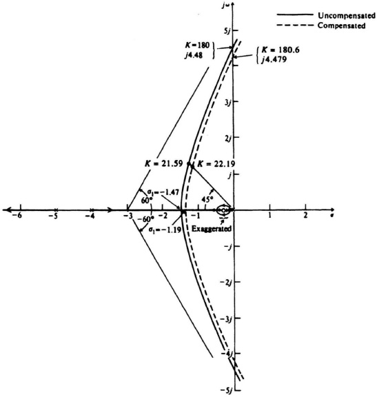
Figure 7.39   Compensation of the root locus shown in Figure 6.57 using a cascaded phase-lag network and an increase in gain.

Let us assume that the combined transfer function representing the increase in gain (n) and the phase-lag network is given by

The form of Eq. (7.123) indicates that this compensator provides a low-frequency gain of n in addition to the phase lag, where n is also the ratio of the break frequencies. The open-loop transfer function of the compensated system is given by

In general, the distances of nα and α from the origin in the s-plane are chosen to be small compared with the distances of the other zeros and poles of the uncompensated open-loop transfer function, so that the added pole and zero of the compensator will not contribute significant phase lag in the vicinity of the gain crossover frequency. This result is quite clear from a study of the Bode diagram, which we shall shortly do at the conclusion of this design (see Figure 7.40). Certainly we do not wish to add the phase-lag contribution in the vicinity of the gain crossover frequency. Therefore, the combination of pole and zero will be quite close together on the root locus and very close to the origin. The combination is usually called a dipole.

In order to complete the design, α is chosen close to the origin at 0.01 and n is chosen, using the following derivation, to achieve a K_v = 30:

Substituting Eq. (7.124) into Eq. (7.125), we obtain

or

Because we desire that K = 21.59 from a transient viewpoint, we must have

The completed root locus for the compensated system whose open-loop transfer function is given by

must now be determined. Because the dipole is added near the origin, the original root locus is not changed significantly, because the two poles and the zero near the origin tend to merge into a single pole.

Let us next determine the new resulting root locus, which is shown as the dashed curve in Figure 7.39, and analyze the effect of the dipole on it. Specifically, we wish to know whether the new root locus will indeed have K_v = 30. In addition, we would like to determine the transient response of the compensated system. Each of the 12 rules for constructing the root locus will be considered.

Rule 1. There are four separate branches, because the characteristic equation,

1 + G(s)H(s) = 0,

is a fourth-order equation.

Rule 2.  The root locus starts (K = 0) from the poles located at the origin, −0.01, −4, and −5. One branch terminates (K = ∞) at the zero located at −0.2779 and the other three branches terminate at zeros which are located at infinity.

Rule 3.  Complex portions of the root locus occur in complex-conjugate pairs.

Rule 4.  The portions of the real axis between the origin and −0.01, −0.2779 and −4, and −5 to −∞ are parts of the root locus.

Rule 5.  The four branches approach infinity as K becomes large at angles given by

Rule 6.  The intersection of the aymptotic lines and the real axis occurs at

Rule 7.  The point of breakaway from the real axis can be computed from the following equation:

(β₁ − β₂ − β₃ − β₄ − β₅)= (2n + 1)π,

where

β₁ = angle from the zero at −0.2779 to the point s₁ that is located a small distance δ off the positive real axis,

β₂ = angle from the pole at the origin to the point s₁,

β₃ = angle from the pole at −0.01 to the Points s₁

β₄ = angle from the pole at −4 to the point s₁,

β₅ = angle from the pole at −5 to the point s₁.

The equation of the transition of the root locus from the real axis to a point s₁ which is a small distance δ off the axis is given by

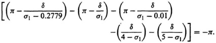
Solving, we obtain σ₁ = −1.19, which compares with a value of −1.47 obtained from Eq. (6.151) for the uncompensated system.

Rule 8. The intersection of the root locus and the imaginary axis can be determined by applying the Routh–Hurwitz stability criterion to the characteristic equation

s(s + 0.01)(s + 4)(s + 5) + K(s + 0.2779) = 0,

which becomes

s⁴ + 9.01s³ + 20.09s² + (K + 0.2)s + 0.2779K = 0.

The resulting Routh–Hurwitz array is given by

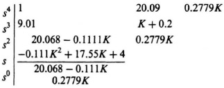
An interesting situation occurs in this Routh–Hurwitz array, because the first terms of the third and fourth rows can go to zero for certain values of gain, K. When the equation

20.068 − 0.1111K = 0

is satisfied, then a possible solution is

K_max = 180.6.

When the equation

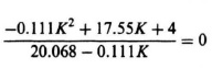
is satisfied, then a possible solution is

K_max = 158.25.

Therefore, in order to find which is (or are) valid, let us substitute s = jω into the characteristic equation and find out where the root locus crosses the imaginary axis. The results can be separated into a real and imaginary part and written in the following form:

For K to be real and imaginary parts of this equation must each equal zero. Therefore, from the imaginary part:

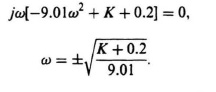
Now, to find the value of K which corresponds to this value of crossing of the imaginary axis, let us substitute this value of ω into the real part of Eq. (7.128). The result is the following equation:

K² − 180.33K − 36.16 = 0.

Therefore, we find that

K = 180.6

is the only possible real value of gain when the root locus crosses the imaginary axis. The analysis indicates that the maximum value of gain, before the system becomes unstable, is 180.6. In Eq. (6.155), we found that the uncompensated system had a maximum allowable gain of 180. Therefore, this result indicates that the dipole has an effect on the maximum allowed gain. The corresponding value of s occuring at the crossing of the imaginary axis is found to be ± j4.479 by substituting K_max into the equation for ω. This compares with a value of s = j4.48 obtained previously for the uncompensated case [see Eq. (6.156)].

Rule 9. This rule does not apply to this problem.

Rule 10. This rule shows that as certain of the loci turn to the right, others turn to the left to ensure that the sum of the roots is a constant.

Rule 11. This rule is quite important to us in this case, because we want to determine the value of gain when ζ = 0.707 (the intersection of a line making an angle of +45° with the negative real axis and the dashed curve). For the uncompensated case, we found that K = 21.59. The new value can be obtained from the following expression:

Measuring the distance from the various poles and zeros to the point of interest, we obtain

K = 22.19.

Therefore, the gain has increased slightly from 21.59 to 22.19. This will result in a slight increase of K_v from 30 to 30.8.

Rule 12. The root locus does not cross itself.

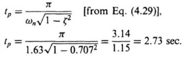
To conclude this problem, we can calculate the value of the time to the first peak and the maximum percent overshoot from Eqs. (7.119) and (7.120), respectively. These results can then be compared with the values obtained from Eqs. (4.29) and (4.33), which assumes that the transient response is completely controlled only by the pair of complex-conjugate poles located closest to the origin. The time to the first peak of the compensated system can be calculated from Eq. (7.119). In order to use this equation, the location of the other two roots must be determined. Using the computer programs (see Sections 6.17 and 6.18) for determining the root locus, these were found to be located at −6.45 and −0.26. Therefore,

where

        ζ = 0.707,

     ω_n = 1.63 (distance from the origin of the complex plane to the two
dominant poles located at 1.15 ± j1.15—dashed curve of Figure 7.39),

= 141° = 2.47 rad,

= 136° + 90° + 14° = 240° = 4.19 rad.

Substituting these values into the equation for t_p, we obtain

Therefore, the time to the first peak is 2.86 sec. If one simply assumes that the transient response is governed by the pair of complex-conjugate poles located at 1.15 ± j1.15 and uses Eq. (4.29) to determine the time to the first peak, then the following is obtained:

Therefore, we see the slightly improved accuracy obtained using Eq. (7.119).

A similar analysis of the uncompensated system, utilizing Eq. (7.119), results in a time to the first peak of 2.81 sec. For this case, the two complex-conjugate poles are located at −1.2 ± j1.2. The third root can be determined analytically from rule 10:

Therefore,

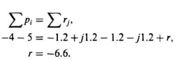
where

         ζ =0.707,

      ω_n = 1.7 (distance from the origin of the complex plane to the two dominant poles—solid curve of Figure 7.39),

= 0,

= 90° + 13° = 103° = 1.8 rad.

Hence,

Observe that the dipole compensation increases the time to the first peak slightly.

The maximum percent overshoot of the compensated system can be obtained from Eq. (7.120). To use this equation, we have to determine the location of the other two roots. As mentioned previously, these were found to be at −6.45 and −0.26. Therefore,

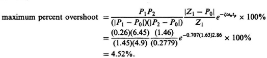
Therefore, the resulting maximum percent overshoot is only 4.52%. If one simply assumes that the transient response is governed by the pair of complex-conjugate poles located at 1.15 ± j1.15 and uses Eq. (4.33) to determine the maximum percent overshoot, then the following is obtained:

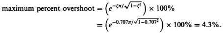
Therefore, we see the slightly increased accuracy obtained using Eq. (7.120).

A similar analysis of the uncompensated system utilizing Eq. (7.120) results in a maximum percent overshoot of 4.48%; for this case, the third root is located at −6.6 as illustrated before:

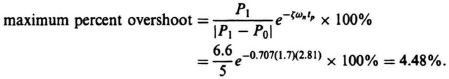
Observe that the dipole compensation increases the maximum percent overshoot slightly.

The results of the transient analysis indicate that the effect of the dipole is to increase the time to the first peak slightly and to increase the maximum overshoot slightly. Of most importance, the dipole increases the velocity constant greatly, from 1.08 to 30.8.

One should note that the dominant pole concept is very useful here, the results coming quite close to the more accurate calculation. In fact, due to the ever-present uncertainty of the parameters of the actual system, it is rarely, if ever, necessary to carry out the detailed calculations indicated.

D.  Comparison of the Root-Locus Method with Bode Diagrams

In our analysis of the system whose transfer function was given by Eq. (7.121) and illustrated in Figure 7.39 using the root-locus method, it was pointed out that this same system’s analysis using the Bode diagram would be very interesting. It is always interesting to compare the analysis of a system using more than one of the techniques shown as was discussed in Section 6.20, where 12 commonly used transfer functions were compared from the viewpoints of the Nyquist-diagram, Bode-diagram, Nichols-chart, and root-locus methods. In this problem, it is especially useful because the root-locus solution may be difficult to comprehend initially. What did we really do when we kept the dominant complex-conjugate roots almost fixed, increased the gain and added a phase-lag network? It is very clear if we look at the uncompensated and compensated systems from the viewpoint of the Bode diagram. For purposes of the Bode-diagram analysis, the value of K in Eq. (7.121) is set equal to 21.59, and this equation is modified to the following easier form for a Bode diagram:

The Bode diagram of the uncompensated system is shown in Figure 7.40. This Bode diagram was obtained using MATLAB (see Section 6.8) and is contained in the M-file part of my MCSTD Toolbox disk and can be retrieved free from The MathWorks, Inc. anonymous FTP server at ftp://ftp.mathworks.com/pub/books/shinners. Notice from this diagram that this system has a gain crossover frequency of 1.025 rad/sec, a phase margin of 64.04°, and a gain margin of 18.42 dB (phase crossover frequency occurs at 4.472 rad/sec). Extension of the initial −20-dB/decade slope intersects the 0-dB line at 1.08 rad/sec indicating a K_v of 1.08 which agrees with Eq. (7.122). (The actual curve intersects the 0-dB line at 1.025 rad/sec.) We now wish to plot the Bode diagram of the compensated system whose transfer function is given by Eq. (7.127). We let K = 22.19 and modify Eq. (7.127) into the following equation which is easier to use for the Bode diagram:

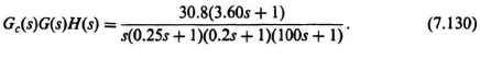
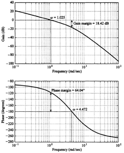
Figure 7.40   Bode diagram for the uncompensated system whose root locus is shown in Figure 7.39.

The resulting Bode diagram for the compensated system, also obtained using MATLAB, whose transfer function is given by Eq. (7.130) is shown in Figure 7.41. It has a gain crossover frequency of 1.138 rad/sec which is close to that of the uncompensated system whose Bode diagram is shown in Figure 7.40 (1.025 rad/sec), because we hardly moved the dominant complex-conjugate poles (see Figure 7.39) in going from the uncompensated to the compensated system. The phase margin of the compensated system is 49.21° (compared to 64.04° of the uncompensated system), and the gain margin of the compensated system is 16.67 dB (compared to 18.42 dB of the uncompensated system). Therefore, the uncompensated system and the compensated system have almost the same relative stability, and about the same gain crossover frequency. From the root-locus viewpoint, this means that the damping factor has hardly changed in going from the uncompensated to compensated systems. (Figure 7.39 shows that the damping factor remains constant at 0.707). However, the velocity constant of the compensated system is 30.8 [see Figure 7.41] compared to the velocity constant of the uncompensated system which is 1.08 [see Eq. (7.122)). In conclusion, the comparison of the stabilization of this problem using the root locus (Figure 7.39) and the Bode diagram (Figures 7.40 and 7.41) is very interesting as the information shown in the root-locus and Bode diagrams complement each other.

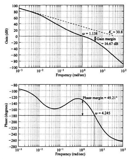
Figure 7.41   Bode diagram for the compensated system whose root locus is shown in Figure 7.39.