6.18.  DIGITAL COMPUTER PROGRAM FOR OBTAINING THE ROOT LOCUS

For those who do not have access to MATLAB, which has now become an industry standard (more or less), this book also provides another digital computer program for obtaining the root locus. This approach for providing both MATLAB and other digital computer programs which are not dependent on COTS (commercial-off-the-shelf software) is used throughout this book.

The root locus can be plotted automatically using a variety of methods, including utilizing a digital computer [29–31]. This section presents a working digital computer program for obtaining the root locus. In our discussions, we will only consider the case of negative feedback. The program can be modified with a few simple changes for positive feedback.

The digital computer is a very versatile and flexible tool that is easily adaptable for automatically determining the roots in the complex plane. The method preseted, based on the material of References [29–31], starts at the poles of the control system and searches for the overall root locus in a segmented manner.

Reference [29] discusses this conceptual algorithm for obtaining the root locus using a digital computer. It presents the logic that can be used to code a digital computer in order to determine the locus of points which satisfy Eqs. (6.132), (6.133), (6.151). The program presented in this section is written in Fortran IV.

The computer logic flow diagrams of the technique are illustrated in Figures 6.70a–d and f. The basis of the conceptual algorithm is a convergent trial-and-error procedure for progressing from a known point on the root locus to a succeeding point. Initial points for the algorithm can be determined by realizing that the locus begins at the poles where the loop gain equals zero. For poles located on the real axis, the locus will remian on it until some breakaway point is reached. For these loci, it will be necessary to determine the breakaway points and begin a search in the complex plane from these points. Terminating points of the root locus are zeros that are located at some finite value or at infinity. Therefore, it is necessary to test and deterine if a locus point is near a zero or if it appears to be heading away from the origin of the complex plane.

The procedure determines the root locus in segments that are ultimately joined together. The process is composed of the following six phases:

(a)  Input and initialization—Figure 6.70a.

(b)  Determine locus segments on real axis—Figure 6.70a.

(c)  Determine breakaway and break-in points of root locus from real axis in positive (upper) half of complex plane—Figure 6.70b.

(d)  Search for root loci which begin at poles/zeros in positive (upper) half of complex plane—Figure 6.70c.

(e)  Search for root loci which begin at poles/zeros on real axis and subsequently enter the positive (upper) half of complex plane—Figure 6.70f.

(f)  Reflect the root-locus segments of the positive (upper) half-plane into the negative (lower) half-plane—Figure 6.70f.

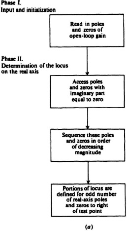
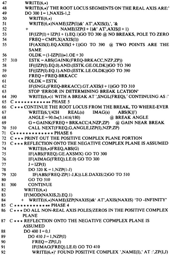
Figure 6.70(a)   Digital computer logic flow chart, phases I and II.

Figure 6.70d illustrates a computer subroutine associated with Figure 6.70c and denoted as “next point.” Let us next consider some of the details associated with each of these computer steps.

The input and initialization phase, illustrated in Figure 6.70a, is concerned with reading in poles and zeros of the open-loop gain.

The second phase of the procedure, denoted as the determination of the locus on the real axis in Figure 6.70a, consists of three sequences. Poles and zeros with imaginary parts equal to zero are determined, and are then sequenced in order of decreasing magnitude. Portions of the locus are then defined for an odd number of real-axis poles and zeros, which exist to the right of a test point.

The third phase, illustrated in Figure 6.70b is concerned with the determination of breakaway and break-in points of the root locus from the real axis in the positive (upper) half of the complex plane. The procedure involves determining the location of the maxima and minima of the function K(σ) as discussed in Rule 7 for construction of the root locus.

Search for root loci which begin/end at poles/zeros in the positive (upper) half of the complex plane, the fourth phase, is illustrated in Figure 6.70c. Successive points of the root locus are determined and the search for additional points are terminated if the following conditions occur:

Figure 6.70(b)   Digital computer logic flow chart, phase III.

(a)  A zero/pole is recognized as the termination of the current locus.

(b)  The termination of the current locus occurs at infinity/zero.

(c)  The current locus intercepts the real axis.

If the last condition occurs, then it is necessary to determine the succeeding behavior of the root locus. In general, the following three situations can occur:

(d)  The locus continues onto the real axis and terminates at a zero/pole on the real axis that is located at a finite value or at infinity.

(e)  the locus continues on the real axis until a breakaway point occurs and it then reenters the full complex plane.

(f)  The locus immediately reenters the imaginary portion of the complex plane.

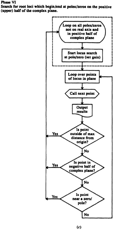
Figure 6.70(c)   Digital computer logic flow chart, phase IV.

Figure 6.70(d)   Digital computer logic flow chart, subroutine.

As each new locus point is obtained, it is examined to determine whether conditions (a), (b), or (c) occur.

Each real-axis intercept should be tested to determine if it lies between the bounds of real-axis root-locus segments determined in the second phase. If it does not, computer error should be noted, and the computer scan should be redone with a higher-accuracy set. Similarly, the real-axis intercepts should be compared with the breakaway points determined in the third phase. If the intercept is not within some small error, then an error condition should be recognized. If more than one break-in point exists at the breakaway point, tests should be made to deterimne which of them has the same slope as the current root locus. If no correspondence is obtained, then an error condition should be recognized.

The root-locus continuation is examined next. A test is made to determine if the root locus can be continued at a nearby zero/pole or a zero/pole located at infinity. If it can, the full locus from start to completion is recorded and displayed. If the root locus reenters the imaginary portion of the complex plane, it will occur at the nearest unassigned breakaway point. The repeated use of “call next point” can then be applied.

The “next point” flow diagram is illustrated in Figure 6.70d. The real and imaginary parts of the point in the complex plane are treated in a real two-dimesional space. An estimate is made of the continuation of the root locus. The initial trial locus point is obtained by computing the intersection of the estimated root-locus continuation with a circle having a small radius r_Δ, as illustrated in Figure 6.70e. There will be two intersecting points and the computer logic must be able to differentiate between them. The net angle contribution for all poles and zeros is computed at the trial locus point. The difference Δθ is computed and compared with the maximum permissible angular deviation of GH from iπ, _θ. If Δθ_θ, then the angle criterion is satisfied and the value of K required to obtain |GH| = 1 is determined. However, if Δθ > _θ, a new trial locus point must be found. The procedure used is to search for an acceptable solution that falls on the previously defined circle illustrated in Figure 6.70e. In the figure, a test point δ_θ is chosen. The difference of the angular contribution of the poles and zeros from iπ, evaluated at the new test point, is denoted as Δ′θ in Figure 6.70e. The change in the angular error is used to determine a new trial locus point on the circle. For computer simplicity, a simple scan of the unit circle is used. After the location of the point and the value of gain are determined, the computer returns to the main routine.

The fifth phase, illustrated in Figure 6.70f, is to search for root loci that begin/end at poles/zeros on the real axis and subsequently enter the positive (upper) half of the complex plane. Only those as-yet-unassigned breakaway (break-in) points in the same segments as the poles (zeros) which lead into the right half-plane and which are also unassigned, are examined. If an assignment can be made, the continuation of the current root locus is determined. The coding in the box labeled “determine root-locus continuation from pole to zero” is exactly the same as that used in the fourth phase (see Figure 6.70c) that exists outside the dotted lines.

Figure 6.70(e)   Estimated root locus point.

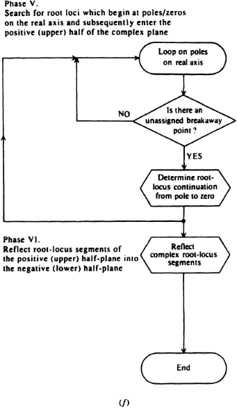
Figure 6.70(f)   Digital computer logic flow chart, phases V and VI [29].

The sixth phase, illustrated in Figure 6.70f is concerned with reflecting the root-locus segments of the positive (upper) half-plane into the negative (lower) half-plane. The fourth and fifth phases of the computer routine are sufficient to have determined all of the root-locus segments in the positive half-plane. Similar segments are also part of the root locus in the negative half-plane.

The computer program written in Fortran for computing the root locus is shown in Table 6.25 and should be compared with the flow charts of Figure 6.70a–f to obtain a thorough understanding of the technique. This program was applied to the root-locus problem analyzed in Figure 6.57 for a system whose transfer function was given by Eq. (6.143). Table 6.26 shows the computer run for the root locus of this system. The results of the computer run are plotted in Figure 6.71. Compare the agreement between the root locus of Figure 6.57 obtained using the construction rules, and the computer-generated root-locus plot of Figure 6.71. It is important to understand the rules of construction and work several examples out using them. After having mastered the technique, it is recommended that this program, or one of the many commercially available programs for plotting the root locus or MATLAB, which was presented in Section 6.17, be used to plot the root locus. Using the computer programs will save you time and give you a root-locus plot of greater accuracy.