2.16.  APPLICATION OF MASON’S THEOREM AND THE SIGNAL-FLOW GRAPH TO MULTIPLE-FEEBACK SYSTEMS

It is important at this point to differentiate between signal-flow graphs and block diagrams. Basically, the signal-flow graph represents a detailed picture of a system’s topological structure, whereas the block diagram focuses on the transfer functions that comprise the various elements of the system. The signal-flow graph is useful in analyzing multiple-loop feedback systems and in determining the effect of a particular element or parameter in an overall feedback system. Essentially both present the same information in different ways, and Mason’s theorem can be applied to both. However, Mason’s theorem is conventionally used with the signal-flow graph, because the topology is more clearly depicted by the signal-flow graph.

Let us next analyze various control-system configurations, depicted by both their block diagrams and signal-flow graphs, using Mason’s theorem.

Example 1. The signal-flow graph corresponding to the block diagram shown in Figure 2.10 is illustrated in Figure 2.15:

Applying Mason’s theorem to this feedback control system results in the following:

  Δ = 1 − [−G(s)H(s)] = 1 + G(s)H(s)

G_A = G(s)

Δ_A = 1

Therefore,

which agrees with Eq. (2.121) that was derived from block-diagram relationships.

Example 2. Let us consider the feedback control system illustrated in Figure 2.16a which contains two feedback paths. Its corresponding signal-flow graph representation is illustrated in Figure 2.16b.

Applying Mason’s theorem to this control system results in the following:

      Δ = 1 − [−G₁(s)G₂(s)H₁(s) − G₂(s)H₂(s)]

G_A(s) = G₁(s)G₂(s)

    Δ_A = 1

Therefore,

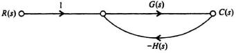
Figure 2.15   Signal-flow graph corresponding to the block diagram shown in Figure 2.10.

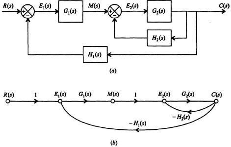
Figure 2.16   Control system containing two feedback paths. (a) Block-diagram representation. (b) Signal-flow graph representation.

Example 3. Let us next consider the feedback control system illustrated in Figure 2.17a which contains four feedback paths. Its corresponding signal-flow graph representation is illustrated in Figure 2.17b.

Applying Mason’s theorem to this control system results in the following:

Δ = 1 − [−G₁G₂G₃G₄G₅G₆G₇G₈H₀ − G₂H₂ − G₄H₄ − G₆H₆].

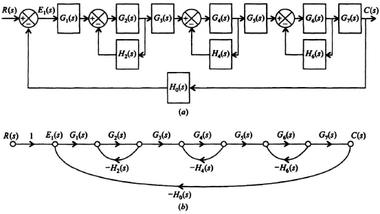
Figure 2.17   Control system containing four feedback paths. (a) Block diagram representation. (b) Signal-flow graph representation.

(All parameters in Δ are functions of s.)

G_A = G₁(s)G₂(s)G₃(s)G₄(s)G₅(s)G₆(s)G₇(s)G₈(s)

Δ_A = 1

Therefore,

(All parameters in C(s)/R(s) are functions of s.)

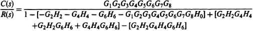
Example 4. For our fourth example, we will analyze the control system whose block diagram is illustrated in Figure 2.11a. Previously, it took us five steps and an entire page of block-diagram reductions to determine C(s)/R(s) using the tedious block-diagram reduction methodology. We will now show how simple the process is using Mason’s theorem which will only require one step for obtaining C(s)/R(s).

The signal-flow graph for Figure 2.11a is shown in Figure 2.18. By inspection, the overall system transfer function is

  Δ = 1 + G₁(s)G₂(s)G₃(s)G₄(s)H₁(s) + G₂(s)G₃(s)H₂(s)
   + G₃(s)G₄(s)H₃(s),

G_A = G₁(s)G₂(s)G₃(s)G₄(s),

Δ_A = 1

Therefore,

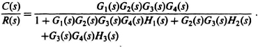
This result agrees with the transfer function shown in Figure 2.11f.

Figure 2.18