5.4.  STATIC ACCURACY

Static accuracy ranks as the next most important characteristics for a feedback control system. The designer always strives to design the system to minimize error for a certain anticipated class of inputs. This section considers techniques that are available for determining the system accuracy.

Theoretically, it is desirable for a control system to have the capability of responding to changes in position, velocity, acceleration, and changes in higher-order derivatives with zero error. Such a specification is very impractical and unrealistic. Fortunately, the requirements of practical systems are much less stringent. For example, let us consider the automatic positioning system of the missile launcher illustrated in Figure 5.1b. Its functioning is similar to the missile launcher positioning system in Figure 1.9. Realistically, it would be desirable for this system to respond well to inputs of position and velocity, but not necessarily to those of acceleration. In addition, it probably would be desirable for this system to respond with zero error for positional-type inputs. However, a finite tracking error could probably be tolerated for inputs of velocity. In contrast to this system, where the stakes are quite high, let us consider a simpler positioning system, which perhaps is only required to reproduce the angular position of a dial at some remote location. Such a control system would probably be only required to reproduce any positional inputs, but not any higher-order inputs such as those of velocity and acceleration.

A method for determining the steady-state performance of any control system is to apply the final-value theorem of the Laplace transform as given by Eq. (2. 74). Let us consider the unity-feedback system shown in Figure 5.2. The relation between the resulting system error, E(s), for a given input R(s) is given by

The steady-state error can be expressed as

The control engineer is usually interested in test inputs of position, velocity, and acceleration. A step, ramp, and paraboloid are simple mathematical expressions which represent these physical quantities, respectively, and is illustrated in Figure 5.3. They are defined in Eqs. (5.10)–(5.12), where the notation U(t) means a unit step for t0:

Figure 5.2   A unity-feedback system.

We next determine the steady-state error of several types of systems for each of these three inputs: the unit step, unit ramp, and paraboloid. It is assumed that the loop transfer function G(s) has the general form

Where

s_n = a multiple pole at the origin of the complex plane,
K = gain factor of the expression.

The term sⁿ in the denominator is of particular significance. It represents the number of multiple poles in the denominator. Based on these number of pure integrations in the denominator of the open-loop transfer function, we classify the system by system “type”. A control system is defined as type 0, type 1, type 2, type 3, ... , if n = 0, n = 1, n = 2, n = 3, ... , respectively. We will show that as the system type is increased, the accuracy is improved. However, the stability problem becomes more difficult as the system type is increased. In practice, we usually never design a control system greater than type 2 because it is very difficult to stabilize a control system containing more than two pure integrations (although it can be done). Therefore, a tradeoff is required between steady-state accuracy and relative stability.

A.  Unit Step (Position) Input

The steady-state error can be obtained by substituting R(s) = 1/s into Eq. (5.9):

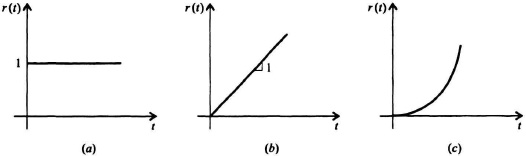
Figure 5.3   Test inputs (a) Unit step representing a position input. (b) Unit ramp representing a velocity input. (c) Parabolic input representing an acceleration input.

The quantity lim_s→0 G(s) is defined as the position constant and is denoted by K_p:

Therefore, the steady-state error in terms of the position constant is given by

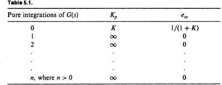
Equation (5.16) states that the steady-state tracking error of a feedback control system having a unit step input equals 1/(1 + the position constant). Table 5.1 summarizes the values of K_p and the resulting steady-state error as a function of the number of pure integrations of the open-loop transfer function G(s).

Table 5.1 indicates that the position constant is infinite for all systems which contian one or more pure integration(s) in the open-loop transfer function G(s). Therefore, Eq. (5.16) implies that all systems containing at least one pure integration result in a theoretical steady-state positional response error of zero. Table 5.1 indicates that the position constant is finite for a system containing no pure integrations and, therefore, the response error for a unit position input is 1/(1 + K).

B.  Unit Ramp (Velocity) Input

The steady-state error can be obtained by substituting R(s) = 1/s² into Eq. (5.9):

The quantity lim_s→0sG(s) is defined as the velocity constant and is denoted by K_v:

Therefore, the steady-state error in terms of the velocity constant is given by

Equation (5.19) states that the steady-state response error of a feedback control system having a unit ramp equals the reciprocal of the velocity constant. Table 5.2 summarizes the values of K_v and the resulting steady-state error as a function of the number of pure integrations of the open-loop transfer function G(s).

Table 5.2 indicates that the velocity constant is infinite for all systems that contain more than one pure integration in the open-loop transfer function G(s). Therefore, Eq. (5.19) implies that al systems containing at least two pure integrations have a theoretical steady-state velocity response error of zero. Table 5.2 indicates that a system containing no pure integrations cannot follow a velocity input. Table 5.2 also indicates that a system containing one pure integration has a response of 1/K due to a unit ramp input.

C.  Parabolic (Acceleration) Input

An expression for the steady-state error due to r(t) = t²U(t) can be obtained by substituting R(s) = 1/s³ into Eq. (5.9):

The quantity lim_s→0 s²G(s) is defined as the acceleration constant and is denoted by K_a:

Therefore, the steady-state error in terms of the acceleration constant is

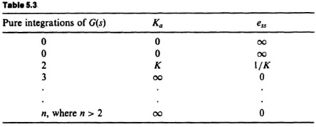
Equation (5.22) states that the steady-state response error of a feedback control system having this parabolic input equals the reciprocal of the acceleration constant. Table 5.3 summarizes the values of K_a and the resulting steady-state error as a function ofthe number of pure integrations of the open-loop transfer function G(s). Table 5.3 inciates that the acceleration constant is infinite for all systems that contain three or more pure integrations in the open-loop transfer function G(s), and the resulting steady-state error is zero. Therefore, Eq. (5.22) implies that all systems containing at last three pure integrations have a theoretical steady-state acceleration response error of zero. Table 5.3 indicates that systems containing less than two pure integrations cannot follow an acceleration input. Table 5.3 also indicates that a system containing two pure integrations has a response error of 1/K for this acceleration input.

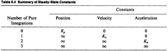
A summary of the results derived appears in Table 5.4. It is quite general and enables the reader to compare the capabilities of various types of systems. Notice from this table that the steady-state constants are zero, finite, or infinite. It is important to emphasize at this time that if the inputs are other than unit quantities the steady-state errors are proportionally increased because we are analyzing linear systems. For example, should the input to a system containing one pure integration be a ramp whose value is B position units (ft/sec, rad/sec, etc.), then the steady-state error as given by Eq. (5.19) would be modified to read

e_ss = B/K_v.

It should be noted that the unit of the velocity constant is 1/sec and that of the acceleration constant is 1/sec². The position constant K_p has no dimensions.

Let us now consider an input composed of position, velocity, and acceleration components which equal AU(t) ft, BU(t) ft/sec, and C/2U(t) ft/sec², respectively. The form of the input can be represented as

r(t) = AU(t) + BtU(t) + Ct²U(t).

The steady-state response of the system may be obtained by considering each component of the input separately, and then adding the results by means of superposition. The resulting steady-state error is of the following form:

It is interesting to see how the various types of systems summarized in Table 5.4 would respond to this input.

1. System Containing No Pure Integration. The steady-state error is

The result indicates that a system containing no pure integration will be able to follow the position input component of AU(t) ft, but not velocity or acceleration inputs of BU(t) ft/sec and C/2U(t) ft/sec², respectively. Figure 5.4 illustrates a typical step response for this system (when there are no velocity or acceleration components in the input).

2. System Containing One Pure Integration. The steady-state error is

e_ss = 0 + B/K_v + ∞.

The result indicates that a system containing one pure integration will follow the position input component with zero error and the velocity input component with a finite error of B/K_v. This system will not, however, be able to follow the acceleration input component. The units of B/K_v are feet or radians. This should be interpreted to mean that there is a fixed positional error due to the constant velocity input component. Figure 5.5 illustrates typical step and ramp responses of this system.

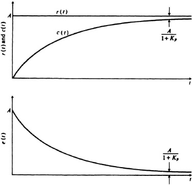
Figure 5.4   Response of a system containing no pure integrations to a step input.

3. System Containing Two Pure Integrations. The steady-state error is

e_ss = 0 + 0 + C/K_a.

The result indicates that a system containing two pure integrations will follow the position and velocity input components with zero error and the acceleration input component with a finite error of C/K_a. The units of C/K_a are feet or radians. This should be interpreted to mean that there is a fixed positional error due to the constant acceleration input component. Figure 5.6 illustrates typical step, ramp, and acceleration responses of this system.

D.  Relationships of Static Error Constants to Closed-Loop Poles and Zeros

It is often important to relate the position, velocity, and acceleration constants to the closed-loop poles and zeros. Let us consider a general single-loop, unity-feedback system having a forward transfer function, G(s), where the closed-loop transfer function is given by

and the relationship between input and error is given by

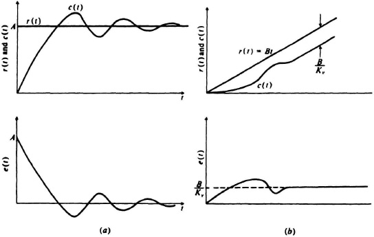
Figure 5.5   Response of a system containing one pure integration to (a) step and (b) ramp inputs.

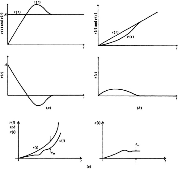
Figure 5.6   Response of a system containing two pure integrations to (a) step. (b) ramp and (c) acceleration inputs.

Because E(s) = R(s) − C(s), it is evident that

It is assumed that C(s)/R(s) can be represented by the rational function

In addition, if 1/[1 + G(s)] in Eq. (5.24) is expanded as a power series in s, the error constants are defined in terms of the successive coefficients:

Now the relationships between K_p, K_v, K_a, and the closed-loop poles and zeros can be determined.

1. Position Constant. Letting s approach zero in Eq. (5.24), we have

Based on the definition of K_p in Eq. (5.15), we can rewrite Eq. (5.27) as

Substituting Eq. (5.28) into Eq. (5.25) with s set at zero, we obtain the following:

Solving for K_p in terms of C(0)/R(0), we have

Using Eq. (5.26a) to represent C(s)/R(s) and letting s approach zero in Eq. (5.26a), we have

Where

product of zeros,

product of poles.

Substituting Eq. (5.30) into (5.29), the following expression for K_p in terms of the closed-loop poles and zeros is obtained:

2. Velocity Constant. In order to derive the velocity constant in terms of the closed-loop poles and zeros, let us substitute Eq. (5.26b) into Eq. (5.25):

Taking the derivative of this expression with respect to s, and then letting s equal zero, we obtain

In addition, we make use of the property that

in unity-feedback systems containing one or more pure integrations. Equation (5.33) says that a closed-loop unity-feedback system behaves with an ideal closed-loop transfer function of one at zero frequency. Dividing Eq. (5.32) by (5.33),

Substituting Eq. (5.26a) into this equation, we have the following:

This can also be written as

or

Therefore. 1/K_v equals the sum of the reciprocals of the closed-loop poles minus the sum of the reciprocals of the closed-loop zeros.

3. Acceleration Constant The acceleration constant in terms of the closed-loop poles and zeros can be derived in a similar manner. We know from Eq. (5.26b) that

From Eq. (5.25), this can be rewritten as

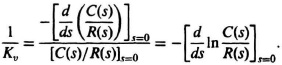
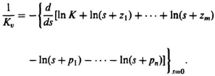
It is obvious from this equation that −2/K_a equals the zero-frequency value of the second derivative of C(s)/R(s). Writing this in terms of the logarithmic derivative:

Setting C(0)/R(0) equal to one, then

Differentiating the right-hand side of Eq. (5.34) and letting s equal zero yields the following expression:

where K_v is defined by Eq. (5.35).

4. An Example. As an example, let us consider the second-order system illustrated in Figure 4.1 whose characteristics are defined by Eqs. (4.1), (4.2), and (4.3):

or

where

This is representative of a wide class of control systems that was thoroughly analyzed in Section 4.2. The problem is to determine K_v in terms of the parameters ζ and ω_n. K_m is the system gain and T_m is the time constant of the open-loop transfer function. The velocity constant of the simple system illustrated in Figure 4.1 is

K_v = K_m

by inspection. Let us relate this velocity constant to ζ and ω_n from the basic definitions of K_m and T_m in terms of ζ and ω_n:

The fact that

is very important to remember for all second-order control systems that are characterized by a pair of complex-conjugate poles. Therefore, in order to obtain very accurate responses to velocity inputs, the damping ratio ζ is made very small. An example of this is in inertial navigation systems where accuracy is much more important than transient responses settling quickly.