7.1.  INTRODUCTION

After the stability of a feedback control system has been analyzed, by using any of the tools presented in Chapter 6, it will often be found that system performances is not satisfactory and needs to be modified. It is necessary to ensure that the open-loop gain is adequate for accuracy, and that the transient response is desirable for the particular application. In order for the system to meet the requirements of stability, accuracy, and transient response, certain types of equipment must be added to the basic feedback control system. We use the term design to encompass the entire process of basic system modification in order to meet the specifications of stability, accuracy, and transient response. The term stabilization is usually used to indicate the process of achieving the requirements of stability alone; the term compensation is usually used to indicate the process of increasing accuracy and speeding up the response.

There are several commonly used configurations for compensating (or stabilizing) a control system. The compensating (or stabilizing) device may be inserted into the system either in cascade with the forward portion of the loop (cascade compensation) as shown in Figure 7.1, or as part of a minor feedback loop (feedback compensation) as shown in Figure 7.2 [1, 2]. The cascade-compensation technique is usually concerned with the addition of phase-lag, phase-lead, and phase-lag–lead passive networks. The feedback-compensation technique is primarily concerned with the addition of rate or acceleration feedback. The type of compensation chosen usually depends on the nonlinearities and the location of the noises in the loop, and economic considerations.

Linear-state-variable-feedback compensation, illustrated in Figure 7.3, consists of feeding back the state variables through constant real gains.

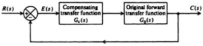
Figure 7.1   Illustration of series or cascade compensation.

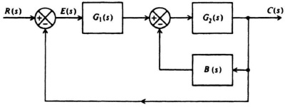
Figure 7.2   Illustration of minor-loop feedback compensation.

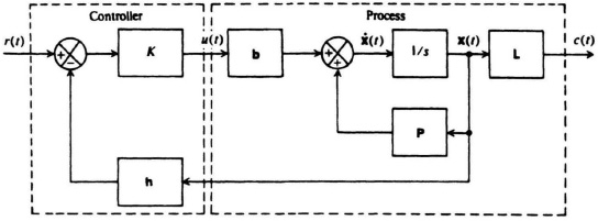
Figure 7.3   Illustration of linear-state-variable-feedback compensation.

Linear-state-variable feedback requires that all state variables be fed back to the controller. For very high-order control systems, it requires a larger number of transducers to sense the state variables for feedback. Therefore, practical applications of this technique can be very costly or impractical. In addition, some state variables may not be directly accessible (e.g., nuclear power plant processes), and this can limit this technique’s application even in low-order control systems. For cases where some state variables may not be directly accessible, we use an estimator to estimate the state variables from measurements made of the accessible variables. Figure 7.4 illustrates an estimator system for a regulator system where the reference input r(t), equals zero.

The compensation techniques illustrated in Figures 7.1 through 7.4 all have only one degree of freedom because there is only one controller in each system, even though the controller can have more than one parameter which can be varied. These one-degree-of-freedom controllers have the major disadvantage that the performance criteria which can be achieved is limited. For example, if a control system is designed to have a desired stability, then it may have poor sensitivity to parameter variations. Let us, therefore, next consider compensation techniques which have two degrees of freedom.

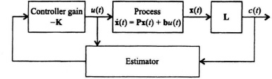
Figure 7.4   Illustration of an estimator system for a regulator system (where the reference input r(t) = 0).

Figure 7.5 illustrates the series-feedback compensation technique in which a series controller and a feedback controller are used. This technique is denoted as having two degrees of freedom compensation because it has two controllers, the series controller G_c(s) and the feedback controller B(s).

Figure 7.6 illustrates forward compensation in which the feedforward controller G_c1(s) is in series with the closed-loop control system which also has a controller G_c2(s) in the forward part of the control system. Because the controller G_c1(s) is not within the feedback loop of the control system, it does not affect the characteristic equation roots of the original control system. Therefore, the poles and zeros of G_c1(s) can be designed to cancel (or add) to the poles and zeros of the closed-loop transfer function. This technique is also referred to as having two degrees of freedom compensation because it has two controllers, the series controller G_c1(s) and the forward-loop controller G_c2(s).

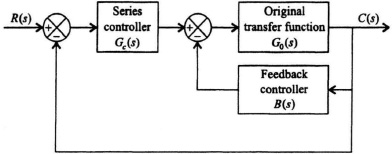
Figure 7.5   Series-feedback compensation technique illustrating two degrees of freedom.

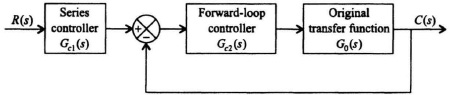
Figure 7.6   Forward compensation with series compensation illustrating two degrees of freedom.

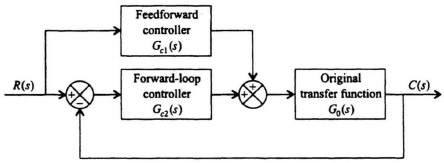
Figure 7.7   Feedforward compensation illustrating two degrees of freedom.

Figure 7.7 illustrates another form of two degrees of freedom compensation system which uses a feedforward controller, G_c1(s), which is placed in parallel with the forward path which contains the controller G_c2(s).

This chapter focuses attention on the tools presented in Chapter 6 which are of practical and useful interest to the control engineer. We will focus our attention on the application of the techniques to those particular design problems they are most suited to solve. Chapter 8 presents modern control-system design techniques using state-space techniques, Ackermann’s formula for pole placement, estimation, robust control, and the H^∞ method for sensitivity reduction. Chapter 6 of the accompanying volume discusses the design of linear feedback control systems from the point of view of modern optimal control theory. Additional linear design problems are presented there in Chapter 7 where actual case studies are presented.