7.2.  CASCADE-COMPENSATION TECHNIQUES

Let us consider the system of Figure 7.1 as our basic starting point in order to analyze the effect of cascade compensation. The compensating transfer function G_c(s) is designed in order to provide additional phase lag, phase lead, or a combination of both at certain frequencies, in order to achieve certain specifications regarding stability and accuracy. We will illustrate and derive the transfer functions for representative compensating passive networks [1–6].

A phase-lag network is a device that shifts the phase of the control signal in order that the phase of the output lags the phase of the input over a certain range of frequencies. An electrical network performing this function was illustrated in Table 2.4 as item 4. Its transfer function was

This can be written in the following more useful form:

Figure 7.8   A complex-plane plot for a phase-lag network.

where

T = R₂C₂,  α = 1 + R₁/R₂.

Observe that αT > T. A complex-plane plot of this network as a function of frequency is shown in Figure 7.8. Notice that the output voltage lags the input in phase angle for all positive frequencies. In addition, observe that the magnitude of E_out(jω)/E_in(jω) decreases from unity at ω = 0 to 1/α at ω = ∞. The Bode diagram for the phase-lag network is illustrated in Figure 7.9. The frequency at which the maximum phase lag occurs, ω_max, and the maximum phase lag, _max, can be easily derived. The results are

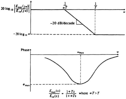
Figure 7.9   Bode diagram of a phase-lag network.

and

Values of _max for certain values of α, which are useful for design purposes, are listed in Table 7.1.

A phase-lead network is a network which shifts the phase of the control signal in order that the phase of the output leads the phase of the input at certain frequencies. An electrical network performing this function was illustrated in Table 2.4 as item 3. Its transfer function was as follows:

This can be written in the following more useful form:

where

Observe that αT > T. A complex-plane plot of this network as a function of frequency is shown in Figure 7.10. Notice that the output voltage leads the input in phase angle for all positive frequencies. In addition, notice that the magnitude of E_out(jω)/E_in(jω) increases from 1/α at ω = 0 to unity at ω = ∞. The Bode diagram for the phase-lead network is illustrated in Figure 7.11. The corresponding values of ω_max and _max for the phase-lead network are

and

Table 7.1.  _max as a Function of α

α	max (degress)
1	0
2	−19.4
4	−36.9
8	−51.0
10	−55.0
20	−64.8

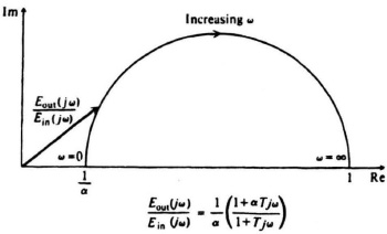
Figure 7.10   A complex-plane plot for a phase-lead network.

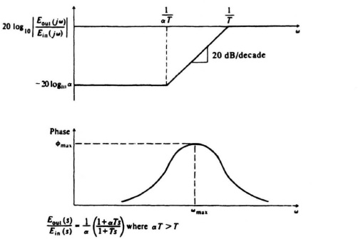
Figure 7.11   Bode diagram of a phase-lead network.

The values shown in Table 7.1 are also true for the phase-lead case except for the sign. An important practical point to emphasize is that the control engineer would not in practice use any ratio of α > 10 because the lead network acts as an attenuation, which must be made up for somewhere in the feedback control system, with an amplification whose ratio is α.

A phase-lag–lead network is a network that shifts the phase of a control signal in order that the phase of the output lags at low frequencies and leads at high frequencies relative to the input. An electrical network performing this function was illustrated in Table 2.4 as item 5. Its transfer function was as follows:

Defining

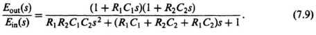
T₁ = R₁C₁.   T₂ = R₂C₂,   T₂₁ = R₁C₂

we can rewrite Eq. (7.9) as

A complex-plane plot of this network as a function of frequency is shown in Figure 7.12. Notice that the output voltage lags the input in phase angle for low frequencies and leads in phase angle for high frequencies. In addition, notice that the magnitude of E_out)(jω)/E_in(jω) decreases for intermediate frequencies and increases to unity as ω approaches 0 and ∞. A corresponding Bode diagram for the phase-lag-lead network is illustrated in Figure 7.13.

Figure 7.12   A complex-plane plot for a phase-lag-lead network.

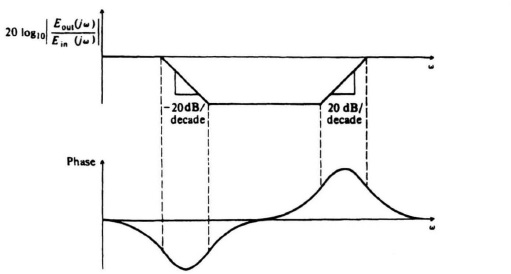
Figure 7.13   Bode diagram of a phase-lag-lead network.

The stabilizing effect of cascaded, phase-shifting networks can easily be demonstrated for a simple second-order system. For example, let us consider the configuration illustrated in Figure 7.1, where the original forward transfer function G₀(s), is given by

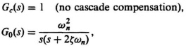
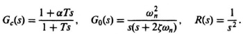
If this system were uncompensated [G_c(s) = 1], then the transfer function G₀(s) would result in the familiar second-order system response which was discussed at great length in Section 4.2. The resulting damping ratio of the system would be given by ζ and its undamped natural frequency by ω_n. Let us now assume that we add a lead network to this system whose transfer function is given by

It is assumed that the attenuation factor of 1/α is compensated for with an amplification increase of α, and the system will maintain the same static error. Let us consider the case where T αT and, therefore, G_c(s) can be approximated by a zero factor (proportional plus derivative control):

Another way of looking at this approximation is the viewpoint of adding a rate feedback loop. In the following section, it is shown in Figure 7.14a that the addition of rate feedback bs in parallel with unity position feedback is equivalent to adding the pure zero factor term (1 + bs) to the open-loop transfer function, G(s)H(s). Therefore, the approximation in Eq. (7.12) can be viewed as an approximate representation of a phase-lead network, or the exact representation of the addition of rate feedback in parallel with position feedback to the system. In the following analysis, we will use the terminology of Eq. (7.12), which is based on an approximation to the phase-lead network, although it could just as easily represent exactly the addition of rate feedback in parallel with position feedback.

The form of Eq. (7.12) suggests that this lead network (or the addition of rate feedback in parallel with unity position feedback) is equivalent to a proportional plus derivative controller. The resulting system transfer function with the lead network is given by

Comparing the denominators of Eqs. (7.13) and (4.3), we observe that it is still of second order and ω_n remains the same, but ζ is greater due to the increase in the coefficient of s in the denominator. The equivalent damping ratio with G_c(s) can be obtained as follows:

Figure 7.14   The stabilizing effects of the systems illustrated are equivalent. (a) Feedback compensation. (b) Cacade compensation—proportional plus derivative controller

where ζ_eq is an equivalent damping ratio with the addition of a zero factor for compensation. Solving for ζ_eq, we obtain

Therefore, we can conclude that the addition of a zero factor in G_c(s) has increased the damping ratio from ζ to ζ_eq by an amount equal to αTω_n/2. This assumes that T is positive, or the zero of the factor (1 + αTs) is in the left half of the s-plane.

The next question is what is the steady-state error resulting from cascade compensation? To answer this, we must find the steady-state errors resulting from the application of a unit ramp input for the cases of no compensation and compare them with those resulting from cascade compensation. We choose a unit ramp as our input because it is the only input which results in a finite response error for a system with a pole at the origin. The transfer function relating error to input for the system shown in Figure 7.1 is given by

Assuming that

and

R(s) = 1/s²  (a unit ramp input),

we find that

Applying the final-value theorem to Eq. (7.17), we find the steady-state error to be

For the case with cascade compensation, a similar analysis yields the following result:

Therefore,

Applying the final-value theorem to Eq. (7.19), the steady-state error is found to be

Comparing the results of Eqs. (7.18) and (7.20), we conclude that the addition of the cascade lead network as given by Eq. (7.11) does not increase or decrease the steady-state response error of the system.

It is important to emphasize that the relationships derived in this analysis apply only to the simple system considered. For example, if a zero factor were contained in the numerator of Eq. (7.10), then these relationships are modified (see Problems 7.5 and 7.6).

If we attempt to extend this analysis of a second-order system to the case of phase-lag compensation, the characteristic equation becomes third order and difficult to factor. For example, if G_c(s) were only to represent the pole factor of the phase-lag network, then

In a similar manner, the closed-loop system transfer function can be found to be given by

The factorization of this characteristic equation is not trivial and a similar analysis to that performed for the phase lead-network case is more complex. The root-locus method is an excellent tool which can be used for factorization, and the analysis of this problem for third- and higher-order systems is presented in Sections 6.14 and 7.9.