7.7.  APPROXIMATE METHODS FOR PRELIMINARY COMPENSATION AND DESIGN USING THE BODE DIAGRAM

Having presented detailed compensation methods, let us next focus our attention on approximate methods for obtaining a first cut at compensation utilizing the Bode diagram [8–10]. Although the procedures presented in this section are approximate, they are generally adequate for the preliminary stage of design. Before the system design is completed, however, the exact magnitude and phase curves should be drawn as indicated previously. The practice of utilizing approximate methods for preliminary design is generally employed as a convenience in obtaining significant time constants, gains, and phase characteristics required for a design.

A.  Approximate Closed-Loop Response from the Bode Diagram

In order to develop the concept of this approach, let us consider the feedback system illustrated in Figure 7.31. The closed-loop transfer of this system is given by

Let us modify this equation into the following more convenient form:

As shown previously, the magnitude (in decibels) of G(s)H(s) can be approximated by straight lines of constant slope when plotted against frequency on a log scale. Therefore, it appears reasonable that the term 1 + G(s)H(s) in Eq. (7.87) may also be dealt with in a similar approximate manner as follows:

Substituting these approximations into Eq. (7.87), we find that

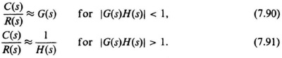
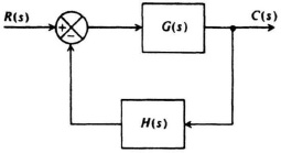
Figure 7.31   A feedback control system.

The approximations of Eqs. (7.90) and (7.91) are very useful as a first cut in the preliminary design of a control system. However, it is important to point out that they are approximate relationships, and are subject to error particularly at those frequencies where G(s)H(s) = 1. However, the amount by which the approximations are in error can be calculated, and this correction can then be applied to correct the approximate value. The resultant corrected value is then an exact solution.

The technique of applying the approximation of Eqs. (7.90) and (7.91) can best be illustrated through an example. Consider the feedback system of Figure 7.31, where

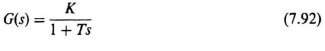
and

This example will illustrate how feedback, around an element containing a time constant, reduces the time constant of that element. Substituting Eqs. (7.92) and (7.93) into Eq. (7.86), the resultant system transfer function is given by

For purposes of illustration, it is assumed that

in this example. For these values, Figure 7.32 illustrates the straight-line approximations for |C(s)/R(s)|, |G(s)|, and |G(s)H(s)|. The dashed curve representing G(s) [and G(s)H(s) as H(s) = 1] has a gain of 10 (20 dB) for frequencies lower than ω = 1/T = 1 rad/sec. At frequencies higher than ω = 1 rad/sec, G(s) and G(s)H(s) have an attentuation of 20 dB/decade. At ω = ω_n = K/T = = 10, G(s) and G(s)H(s) approximately equal 0 dB. Equation (7.91) indicates that for frequencies lower than ω_n = 10, the system transfer function C(s)/R(s) equals 1/H(s) = 1 and is shown by the solid line at 0 dB. For frequencies greater than ω_n, Eq. (7.90) indicates that C(s)/R(s) is equal to G(s) as shown. Figure 7.32 illustrates very clearly that the use of unity-gain feedback around a single time-constant element results in a reduction in its time constant. This admirable characteristic is achieved at the expense of a loss of gain.

It is important to recognize that the results obtained for the closed-loop transfer function are approximate. For example, Eq. (7.94) indicates that the gain is actually K/(1 + K) = 10/(1 + 10) = 0.909 instead of 1 for ω < ω_n, and the closed-loop time constant is T/(1 + K) = 1/(1 + 10) = 0.0909 instead of T/K = = 0.1. Note that these errors decrease as the gain K increases. Generally, K is quite large and the error between the approximate and exact curves is very small.

The form of Eq. (7.87) is very well suited for determining the value of C(s)/R(s) when |G(s)H(s)| > 1, with the bracketed term representing the difference between the approximate and exact curves. In order to determine a general analytic expression for finding the difference between the approximate and exact curves when |G(s)H(s)| < 1, let us reconsider Eq. (7.86) and rewrite it as follows:

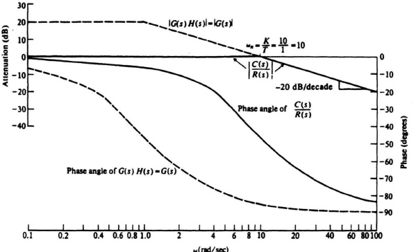
Figure 7.32   Open- and closed-loop gain and phase characteristis for the system of Figure 7.31 where G(s) = 10/(1 + s) and H(s) = 1.

Therefore,

For those frequencies where |G(s)H(s)| < 1, the bracketed term of Eq. (7.98) represents the error between the approximate solution

and the exact solution. Another way of looking at this is that the bracketed term represents a correction factor which can be used to correct the results of the approximation given by Eq. (7.90).

B.  The Straight-Line Phase-Shift Approximation

For preliminary design purposes, it is usually sufficient to obtain quantitative information regarding phase shift without resorting to the exact but tedious method of calculating the phase. We have found it convenient to represent the amplitude characteristics by a straight-line approximation, and can utilize a similar technique for the phase-shift function. In order to introduce the method, let us consider the phase shift due to the transfer function representing a zero factor given by

Figure 7.33a illustrates the exact and straight-line approximation and Figure 7.33b illustrates the exact phase shift and its straight-line approximation. The straight-line approximate phase shift has been constructed by drawing a straight line tangent to the actual curve at ω = ω₁.

In order to construct these straight-line phase-shift approximations by inspection, the dependence of ω_A and ω_B on ω₁ must be known. This can be obtained by first considering the slope of the actual curve at ω = ω₁ as follows:

The slope at ω = ω₁ can be obtained by differentiating this expression:

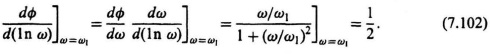
Figure 7.33   Straight-line, approximate, phase-shift methods for a zero factor term.

Knowing the slope at ω = ω₁, the intercepts at ω_A and ω_B can be obtained from

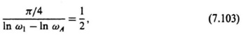
which gives

Therefore,

It is interesting to note that if a number other than e were chosen for the logarithmic base, the slope in Eq. (7.105) would change, but the frequency ratio given by Eq. (7.105) would remain the same.

Based on this result, complicated approximate straight-line phase-shift curves can be obtained. Figure 7.34 illustrates the application of this approach for a transfer function given by

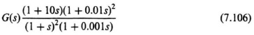
and compares the approximate straight-line phase-shift curve with the exact phase-shift curve. Observe that the errors obtained by using the approximate phase curve are larger than the corresponding errors of the amplitude approximation. However, the use of this approximation greatly aids the control-system engineer in obtaining a first cut preliminary design.

The example just presented contained roots that were all real. What happens if the transfer function contains underdamped quadratic factors? In order to analyze this situation, let us consider the following normalized quadratic phase-lag factor (ζ < 1):

It was shown in Section 6.7 that the amplitude and phase-shift terms are given respectively by [see Eq. (6.92)]:

Figure 7.34   Approximate straight-line phase-shift (solid lines) and exact phase-shrift (short dash–long dash line) characteristics of

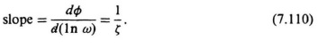
Let us focus attention on the phase-shift term. Differentiation of Eq. (7.109) results in the slope at ω = ω_n, being given by

As before, the two intercepts ω_A and ω_B can be found as follows:

Therefore,

Exact phase characteristics corresponding to Eq. (7.107) and its straight-line approximation, based on the relationship of Eq. (7.112), are illustrated in Figure 7.35. In addition, the exact amplitude characteristics of Eq. (7.108) and its straight-line approximation are also illustrated. Observe from Eq. (7.112) that as ζ approaches zero, the two frequency ratios decrease and approach unity in the limits. This certainly agrees with the exact phase characteristics of a quadratic phase lag as illustrated in Figure 6.28. On the other hand, when ζ = 1, the roots become real and Eq. (7.112) reduces to Eq. (7.105).

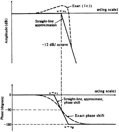
Figure 7.35   Straight-line approximate phase-shift method for a quadratic lag factor (ζ < 1).

The reader is again reminded that the straight-line phase-shift approximation is not exact. It should only be used in order to obtain a first cut for preliminary design work. It shouldalso be noted that the errors of the straight-line phase-shift approximation are generally larger than the corresponding errors of the amplitude approximation. For this reason, the phase-shift approximation is not used for final design. In the final design, the actual phase-shift characteristics must be employed as previously illustrated.