8.2.  POLE-PLACEMENT DESIGN USING LINEAR-STATE-VARIABLE FEEDBACK

Having presented methods for designing linear control systems using classical techniques, let us now look at the problem of specifying pole placement from the viewpoint of state-variable feedback [1]. In order to do this, let us first look at the basic feedback problem illustrated in Figure 8.1. This figure illustrates the concept of feeding back the states of the process in addition to that of the output. Because a linear process can be characterized by the phase-variable canonical equations

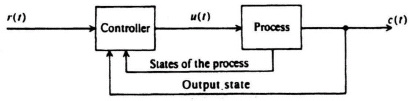
Figure 8.1  General feedback system problem illustrating feedback of the output state and the states of the process.

let us consider the configuration of Figure 8.2. It is important to observe from this figure that the control signal is generated from a knowledge of the reference input r(t) and the state variables x(t). Note that r(t), u(t), and c(t) represent scalars.

In general, the control input u can be represented as

u(t) = f (x(t), r(t)).

Rather than considering the controller in such a broad sense, let us consider the specific condition of linear state-variable feedback where the controller weights the sum of the state variables in a linear manner. In addition, it is assumed that the controller provides a linear gain K which multiplies the difference between the reference input and the linear weighted sum of state variables fed back. Therefore, u(t) can be represented as

where h_i is defined as the ith feedback coefficient. In matrix form, u(t) can be represented as

where

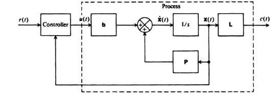
Figure 8.2  General feedback system with state-variable feedback.

Figure 8.3 presents a matrix representation of the concept of linear-state-variable feedback, and Figure 8.4 is an example of a physical representation of a typical system as implied by Figure 8.3. In the following discussion, it is assumed that all state variables are directly available for measurement and control. In practice, this is not always possible, and techniques for modifying and extending the design procedure presented, to the case where all the state variables are not available, are also discussed in Sections 8.6 and 8.7.

How does linear feedback of the state variables affect the behavior of the process given by Eqs. (8.1) and (8.2)? This can easily be determined by substituting Eq. (8.4) into Eq. (8.1):

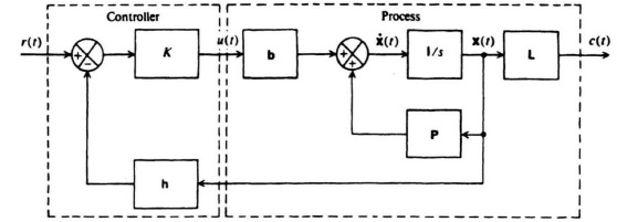
Figure 8.3  Linear-state-variable feedback representation.

Figure 8.4  Example of pole placement design using linear-state-variable feedback.

Simplifying Eq. (8.7), and incorporating Eq. (8.2), we obtain the closed-loop equation

where

is the closed-loop-system matrix. Comparing Eq. (8.1) and (8.2) with (8.8) and (8.9), we observe that they are identical except that the P matrix has been replaced by P_h and u(t) becomes Kr(t).

How can we relate the closed-loop-system matrix P_h to the closed-loop transfer function, C(s)/R(s)? This can be accomplished by taking the Laplace transform of Eqs. (8.8) and (8.9). Because the results will be used to find a transfer function, all initial conditions are assumed to be zero:

Solving for X(s) from Eq. (8.11), we get

The inverse matrix [sI − P_h]⁻¹ is defined as the closed-loop resolvent matrix, Φ_h(s), where

Therefore, Eq. (8.13) may be rewritten as

Substituting Eq. (8.15) into Eq. (8.12), we obtain a relation between C(s) and R(s):

Therefore, the closed-loop transfer function in terms of the closed-loop resolvent matrix is given by

In addition, the characteristic equation in terms of the closed-loop-system matrix can also easily be determined, simply by substituting the numerator and denominator portions of the inverse matrix, Φ_h(s):

The corresponding characteristic equation of the closed-loop system in terms of the closed-loop system matrix is given by

Because we are concerned with synthesizing control systems in terms of pole placement design using linear-state-variable feedback concepts, we would like to force the system illustrated in Figure 8.3 into the generalized form illustrated in Figure 8.5, and study its properties. Let us first consider the derivation of H(s). From Figure 8.5 we observe that

Substituting Eq. (8.12) into Eq. (8.20), we obtain

After substitution of Eq. (8.15) for X(s), Eq. (8.21) becomes

The term G(s) can also be derived in terms of Φ_h(s). The closed-loop transfer function of the system illustrated in Figure 8.5 is given by

Substituting Eqs. (8.17) and (8.22) into Eq. (8.23), we obtain the expression

Combining Eqs. (8.22) and (8.24), the open-loop transfer function is found to be given by

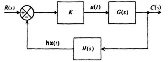
Figure 8.5  An equivalent model of Figure 8.3.

Let us compare Eqs. (8.17), (8.22)–(8.24), and (8.25) in order to draw conclusions regarding G(s), H(s), the open-loop transfer function KG(s)H(s), and the closed-loop transfer function C(s)/R(s). These characteristics will be important for designing systems using pole placement techniques with linear-state-variable feedback techniques in the following section. Based on these five equations, we can state the following properties:

1. The poles of KG(s)H(s) are the poles of G(s).
2. The zeros of C(s)/R(s) are the zeros of G(s).
3. The pole-zero excess of C(s)/R(s) must be equal to the pole-zero excess of G(s).

With these properties as a basis, we consider in the following section the design of control systems from the viewpoint of linear-state-variable feedback.