
PROBLEMS
6.1. The stability of the feedback control system of Figure P6.1 is to be determined.

Figure P6.1
(a) Determine the system’s P matrix from its state equations.
(b) Find the system’s characteristic equation from knowledge of the P matrix.
(c) Using the Routh–Hurwitz criterion, determine whether this feedback control system is stable.
6.2. Stability of the control system of Figure P6.2 is to be determined.

Figure P6.2
(a) Determine the system’s P matrix from its state equations.
(b) Determine the characteristic equation of this system from knowledge of the P matrix.
(c) Utilizing the Routh–Hurwitz criterion, determine the necessary relationship between T1 and T2 for this system to be stable.
6.3. A feedback control system can be represented by a state vector differential equation where
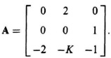
(a) Determine the characteristic equation of this control system.
(b) Using the Routh–Hurwitz criterion, determine the range of K where the system is stable.
6.4. Consider the control system of a tracking radar system which operates in two coordinate axes. Its signal-flow graph, which is illustrated in Figure P6.4 indicates that there is electrical coupling between the control systems for the two axes:
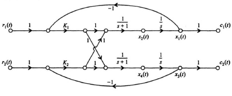
Figure P6.4
(a) Determine the phase-variable canonical equations for this control system.
(b) Determine the characteristic equation of this system.
(c) Is the system stable?
6.5. Phase-locked loops maintain zero difference in phase between an input carrier signal and a voltage-controlled oscillator. They are used in various applications including television, space telemetry, and missile tracking systems. The block diagram in Figure P6.5 is a linearized approximation of a specific phase-locked loop used for a space telemetry application:
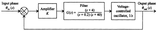
Figure P6.5
(a) Determine the maximum value of K so that this phase-locked loop is stable.
(b) The control system engineer designing this phase-locked loop also has a system requirement in this application that the steady-state error of the system shall be one degree for a ramp signal change of 10 rad/sec. Determine the value of K to meet this specification. Is this value of K within the allowable range of gain found in part (a) for which the system is stable?
6.6. A control system used to position a load is illustrated in Figure P6.6.
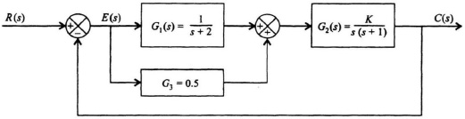
Figure P6.6
(a) Determine the characteristic equation of this control system.
(b) Determine the maximum value of K which can be used before the system becomes unstable using the Routh–Hurwitz criterion.
6.7. The field of fluidics is relatively new [49]. The use of fluids as a power source is not new, but the discovery that this energy can be manipulated and utilized in much the same way as electricity, and without the need for moving parts, has sparked the technology of fluidics. The term fluidics refers to the field of technology that is concerned with the use of either liquid or gaseous fluids in motion to perform functions such as amplification, sensing, switching, computation, and control. These systems have the advantages of high reliability, operation under extreme environmental conditions, resistance to radiation, and low cost. Fluidic control systems are especially applicable to fluid-flow systems, such as those using a turbine. Figure P6.7 illustrates the equivalent block diagram of a fluidic speed-control system. Actual speed, derived from a tuning-fork device, is compared with the desired speed. Any difference is amplified by a fluidic amplifier, which then activates a valve used to control the turbine’s speed.
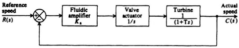
Figure P6.7
(a) Determine the state-variable signal-flow diagram and the phase variable canonical equations of this system when Ka = 10 and T = 100.
(b) Determine the characteristic equation of this system from the relation |P − sI| = 0.
(c) Utilizing the Routh–Hurwitz criterion, determine whether the system is stable.
6.8. Using the Routh–Hurwitz stability criterion, determine if the feedback control system shown in Figure P.68 is stable for the following transfer functions:

Figure P6.8
(a) ![]()
(b) ![]()
(c) ![]()
(d) ![]()
6.9. Figure P6.9a illustrates the submarine depth-control problem. The object is to adjust the actual depth C to equal a desired depth R. The control system depends on a pressure transducer, which is used to measure the actual depth. Any difference between the actual and desired depths is amplified and is used to drive the stem plane actuator through an appropriate angle θ until the actual depth equals the desired depth. An equivalent block diagram of such a system is illustrated in Figure P6.9b. Utilizing the Routh–Hurwitz criterion, determine whether this system is stable for the parameters indicated.

Figure P6.9 (a) Submarine depth-control problem. (b) Block diagram of system.
6.10. Using the Routh–Hurwitz stability criterion, determine whether the feedback control system illustrated in Figure P6.10 is stable.

Figure P6.10 Feedback control system.
6.11. Automatic control systems are being used to an ever-increasing degree in the railroad transportation field [50]. A very widely acclaimed high-speed rail transportation system is in operation in Japan [51]. Figure P6.11a is a photograph of the Shinkansen Tokyo-to-Osaka railroad, which is commonly referred to as the Tokaido line. Figure P6.11b illustrates an equivalent block diagram for the automatic braking system used to regulate this class of high-speed train.
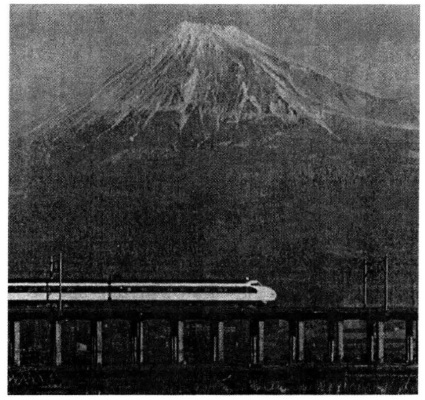
Figure P6.11 (a) Shrinkansen Tokaido line. [Courtesy of Japan National Tourist Organization (JNTO)]

Figure P6.11 (b) Block diagram: automatic braking system.
(a) Determine the signal-flow graph and the characteristic equation of this system.
(b) Using the Routh–Hurwitz criterion, determine the allowable values of amplifier gain Ka for system stability. Assume the following parameters:
K1 = 1, K2 = 1000, K3 = 0.001,
a = 0.1, b = 0.1.
6.12. Using the Routh–Hurwitz stability criterion, determine whether the feedback control system illustrated in Figure P6.12 is stable.
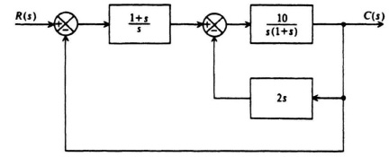
Figure P6.12
6.13. The tool of mathematical modeling can be used to study economic problems of a much larger scope than that found in a single business organization. The economics concerned with national income, government policy on spending, private business investment, business production, taxes, and consumer spending may be represented [49] by the block diagram of Figure P6.13. Although business production lags available funds according to a pure time delay, the representation of Gs(s) by the lag factor 1/(1 + Ts), is adequate. Assuming that E(s) and U(s) are related by
U(s) = −(A + Bs)E)s),
and government policy is represented by
G1(s) = C + Ds,
determine the requirements on C and D in terms of A and B for system stability.

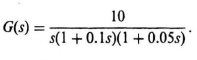
6.14. By means of Nyquist-diagram plots, determine whether feedback systems represented by the following values of G(jω)H(jω) are stable.
(a) ![]()
(b) ![]()
(c) ![]()
(d) ![]()
Do not attempt to plot the exact values of G(jω)H(jω) for all values of frequency. It should only be necessary to determine a few values of frequency exactly.
6.15. By means of a Nyquist-diagram plot, determine whether the system illustrated in Figure P6.15 is stable.
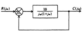
Figure P6.15
6.16. Determine whether the system illustrated in Figure P6.16 is stable by means of a Nyquist-diagram plot.
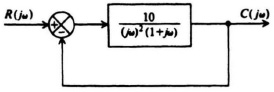
Figure P6.16
6.17. The Nyquist diagram for a control system is as shown in Figure P6.17.
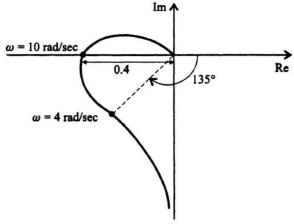
Figure P6.17
The control system is known to have an open-loop transfer function whose form is given by the following:
![]()
Determine the values of K1, K2, and K3.
6.18. The Nyquist diagram of a control system is illustrated in Figure P6.18. This control systems’s open-loop transfer function, G(s)H(s), does not have any poles in the right half-plane. Determine whether the system is stable or not, and determine the number of roots (if any) which are located in the right half-plane.
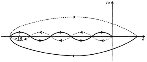
Figure P6.18
6.19. The positive-frequency portions of the Nyquist diagram for several transfer functions are shown in Figure P6.19. Complete the Nyquist diagram and determine stability, assuming that G(jω)H(jω) has no poles in the right half-plane.
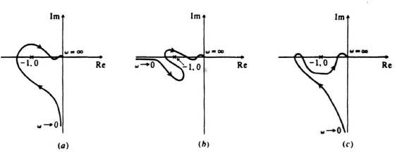
Figure P6.19
6.20. The design of automatic control systems for electronic activation of human limb movements is an interesting example of the application of control theory [52]. By means of electrical pulses, a paralyzed limb can be made to contract, with the result that functional movements of the extremity are performed. Figure P6.20a illustrates the concept implemented using conventional control-system techniques. The electronic controller G(s) feeds electrical signals to the contracting muscles (agonists), which stretch the opposing muscles (antagonists). Figure P6.20b illustrates the equivalent block diagram where the following transfer functions can be assumed:
G(s) = A,
Typical values of the parameters are as follows:
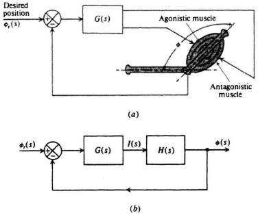
Figure P6.20
J= 1, C = 20, τ0 = 0.1, K′ = 1.
(a) Utilizing the Nyquist diagram, determine the phase margin when the electronic gain A is set at 2.
(b) Repeat part (a) when the electronic gain is set at 100.
6.21. A unity negative-feedback control system’s forward transfer function is given by the following:
![]()
(a) Sketch the Nyquist diagram for this control system.
(b) Is the resulting system stable or unstable? If it is unstable, determine the number of roots in the right half-plane.
6.22. A feedback control system has the configuration shown in Figure P6.22.
(a) Draw the Nyquist diagram of the loop gain function.
(b) Draw the Bode diagram showing the magnitude, in decibels, and phase angle, in degrees, as a function of frequency.
(c) Find the phase margin and gain margin of the system. Illustrate these points on the graphs for parts (a) and (b).
(d) Find the values of Kp, Kv, and Ka.
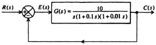
Figure P6.22
(e) What is the steady-state velocity-lag error for a velocity input of 5 rad/sec?
6.23. A unity negative-feedback control system’s forward transfer function is given by the following:
![]()
(a) Sketch the Nyquist diagram for this control system.
(b) Is the resulting system stable or unstable? If it is unstable, determine the number of roots in the right half-plane.
6.24. A feedback control system has the configuration shown in Figure P6.24.
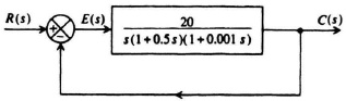
Figure P6.24
(a) Plot the Bode diagram for this system.
(b) What is the gain crossover frequency? What is the phase margin at gain crossover? What is the gain margin? Is the system stable?
(c) Find the values of Kp, Kv, Ka.
(d) What is the steady-state velocity-lag error for a velocity input of 40 rad/sec?
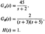
6.25. Draw the straight-line attenuation diagrams, showing the magnitude in decibels, and the phase characteristics, showing the phase angle in degrees, as a function of frequency, for the following transfer functions:
(a) ![]()
(b) ![]()
(d) ![]()
Assuming that GA(s) and GC(s) represent open-loop transfer functions of unity-gain feedback systems, determine the phase and gain margins in parts (a) and (c).
6.26. We wish to design the control system shown in Figure P6.26 so that the phase margin is 70°.

Figure P6.26
Without using semi-log graph paper, determine analytically the value of the amplifier gain K so that the phase margin is 70°.
6.27. An engineer is called in to consult on a control system in a piece of equipment in the field. No one can find the design report or test results from the original design of the control system. The engineer, therefore, decides to take a frequency response of the control system by opening up the outer feedback loop. The resulting asymptotic gain–frequency characteristic is obtained as shown in Figure P6.27.
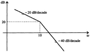
Figure P6.27
Assuming that the system is a minimum-phase transfer function, determine the transfer function, G(s)H(s).
6.28. A tank-level control is shown in Figure P6.28. It is desired to hold the tank level C within limits even though the outlet flow rate V1 is varied. If the level is not correct, an error voltage En is developed which is amplified and applied to a servomotor. This in turn adjusts a valve through appropriate gearing N and thereby restores balance by adjusting the inlet rate, M2.

Figure P6.28
The following relations are valid from this figure:
En = R − C = error in level (in),
E0 = KaEn = voltage applied to motor (volts),
M1 = G1(s)E0 = valve position (rad),
M2 = KvM1 = tank feed flow (ft3/sec),
C = G2(s)M2 = tank level (in).
The pertinent constants and transfer functions are as follows:
G1(s) =
rad of valve motion per volt,
G2(s) = 0.5/s in of level per ft3/sec,
Kv, = 0.1 ft3 sec per rad of valve motion,
Ka = amplifier gain to be set,
Error detector sensitivity = 10 V per in of error.
(a) Draw the system block diagram showing all transfer functions.
(b) Using a Bode diagram for the solution, determine the amplifier gain Ka required to meet a required gain crossover frequency of 1.5 rad/sec.
(c) With the gain set at the value determined in part (b), what are the resulting phase and gain margins?
6.29. By utilizing automatic ship steering systems, a ship can maintain a desired heading much more accurately than if it depended on a helmsman correcting the heading at infrequent intervals. Accurate ship heading is a particular crucial problem for minesweepers who must sweep desired, prescribed, straight paths with very little allowable deviations. Figure P6.29 illustrates the overall control problem where δ represents the deviation of the mine sweeper from the desired heading and θ represents the angle of deflection of the steering rudder. The transfer function relating θ(s) and δ(s) for a 180-ft minesweeper moving at 13 ft/sec is given by [53]
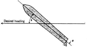
Figure P6.29
![]()
Determine the Bode diagram for this transfer function.
6.30. Repeat Problem 6.22 for the transfer function
![]()
6.31. A feedback control system has the configuration shown in Figure P6.31, where U(s) represents an extraneous signal appearing at the input to the plant.

Figure P6.31
(a) Assuming that G1(s) = 1, plot the decibel-log frequency diagram and the phase diagram for this system.
(b) It is desired that the steady-state error resulting from an extraneous unit step input signal at U(s) shall be 0.1 unit. Assuming G1(s) = K, determine K to meet this specification.
(c) Determine the gain crossover frequency, phase margin, and gain margin resulting from part (b).
6.32. A feedback control system has the configuration shown in Figure P6.32.

Figure P6.32
(a) Plot the Bode diagram for this system.
(b) What is the gain crossover frequency? What is the phase margin at gain crossover? What is the gain margin? Is the system stable?
(c) Find the values of Kp, Kv, Ka.
(d) What is the steady-state velocity-lag error for a velocity input of 40 rad/sec?
6.33. Repeat problem 6.28 with an error-detector sensitivity of 1 V per inch of error.
6.34. Repeat Problem 6.31 with the transfer function of G2(s) given by

6.35. A second-order servomechanism has a forward transfer function given by
![]()
The feedback transfer function is unity.
(a) Draw the Bode diagram showing the magnitude and the phase characteristics as a function of frequency.
(b) Using the Nichols chart, plot a curve of frequency response of the closed-loop system.
(c) What are ωp and Mp?
(d) Can this system ever be unstable no matter how large the forward gain is made? Explain.
6.36. Repeat Problem 6.35 for
![]()
6.37. Repeat Problem 6.35 for
![]()
6.38. Driving an automobile is a feedback process, as indicated in the block diagram [54] of Figure P6.38.
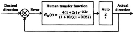
Figure P6.38
The objective of the system shown is for the driver to maintain a desired direction along the road. Any error is sensed by the driver’s eyes and is transmitted to the brain, which then activates his muscles appropriately. With his muscles, the driver controls the steering wheel. The human transfer function shown in the block diagram is based on test data for a particular driver, and is of the same form discussed in Problem 6.64.
Using the Bode-diagram method, determine the phase margin and gain margin that this system has.
6.39. Consider the same feedback control system analyzed in Problem 6.1. Its stability is to be analyzed in this problem using the Bode diagram.
(a) Draw the Bode diagram for this system, both the amplitude and phase diagrams.
(b) Determine the phase and gain margins from your Bode diagram. Is this system stable? (Note: Your answer as to whether the system is stable in this problem should agree with your answer regarding stability in Problem 6.1.)
(c) Repeat parts (a) and (b) if the gain is increased to 200. (Hint: Modify your Bode diagram of part (a) to do this part. Drawing a new Bode diagram is not necessary.)
6.40. The stability of a submarine depth-control system illustrated in Figure P6.40a is to be analyzed using the Bode diagram. In the block diagram of the system illustrated in Figure P6.40b, a pressure transducer measures the actual depth, which is then compared to the desired depth. Any difference between the actual and desired depths is amplified and is used to drive the stern plane actuator through an appropriate angle θ until the actual depth equals the desired depth.
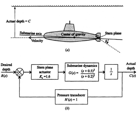
Figure P6.40 (a) Submarine depth-control system (b) Block diagram of the system
(a) Draw the Bode diagram, and find the gain crossover frequency.
(b) Find the phase margin and gain margin of the depth-control system.
6.41. In Figure P6.41a, Astronauts George D. Nelson (right) and James D. van Hoften (left) use the mobile foot restraint and the remote manipulator system (a robot arm-like device) as a “cherry picker” for moving about on the Challenger space shuttle mission, Flight 41-C, on April 11, 1984. They shared a repair task on the “captured” Solar Maximum Mission Satellite in the aft end of the Challenger’s cargo bay. Later, the remote manipulator system lifted the Solar Maximum Mission Satellite into space once more. An approximate equivalent block diagram of this operation, which is illustrated in Figure P6.41b, contains an approximation for modeling the astronaut [54].
(a) Draw the Bode diagram and determine the gain crossover frequency, phase, and gain margins for K = 10.
(b) Repeat part (a) if K is reduced in half to 5.
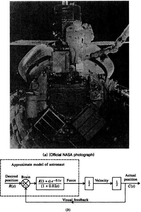
Figure P6.41 (a) Mobile foot restraint and remote manipulator: Challenger space-shuttle Flight 41-c, April 1984 (Official NASA photograph). (b) Block diagram of operation
(c) Repeat part (a) if K is doubled to 20.
(d) What conclusions can you reach from your results?
6.42. A feedback control system has a block diagram as shown in Figure P6.42.
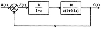
Figure P6.42
(a) Determine the required gain K for a steady-state velocity-lag error of 30° with an input velocity of 10 rad/sec.
(b) What are the values of Mp and ωp?
6.43. A unity-feedback control system has a forward transfer function given by
(a) Plot G(jω)H(jω) on the Nichols chart.
(b) What are the values of Mp and ωp?
6.44. Repeat Problem 6.43 for
![]()
6.45. A unity negative-feedback control system has a forward transfer function given by
![]()
(a) Sketch the root locus giving all pertinent characteristics of the locus.
(b) At what value of gain does the system become unstable?
6.46. Repeat Problem 6.45 for the following transfer functions:
(a) ![]()
(b) ![]()
(c) 
(d) ![]()
6.47. Sketch the root locus for a negative-feedback control system having the following forward and feedback transfer functions:
![]()
6.48. Sketch the root locus of a unity positive-feedback system whose transfer function is given by
![]()
(a) Draw the root-locus diagram of a negative-feedback control system whose feedback-path transfer function is unity and whose forward-path transfer function is given by the following:
![]()
(b) At what value of K does the system become unstable, and where does the root locus intersect the jω axis when this occurs?
6.50. Sketch the root locus for a negative-feedback control system having the following forward and feedback transfer functions:
![]()
6.51. Repeat Problem 6.50 for positive feedback. What conclusions can you draw from your result?
6.52. Draw the root locus of a positive feedback system where
![]()
6.53. Determine the root locus for a feedback system whose open-loop transfer function is given by
![]()
For −∞ ![]() K
K ![]() ∞. Indicate all pertinent values on the root locus.
∞. Indicate all pertinent values on the root locus.
6.54. A negative-feedback system has an open-loop transfer function given by
![]()
(a) Draw the root locus and label all pertinent values on the root locus.
(b) For what range of values of gain is the system stable?
(c) Draw the Bode diagram of the system and correlate the regions of stability and instability with the root-locus results. Assume that K = 1.
6.55. Repeat Problem 6.52 for the case of negative feedback.
6.56. Reconsider the ecological model of rabbits and rabbit-eating foxes presented in Problem 2.72. The state equations of the process were given by
![]() 1(t) = Ax1(t) − Bx2(t),
1(t) = Ax1(t) − Bx2(t),
![]() 2(t) = −Cx2(t) + Dx1(t),
2(t) = −Cx2(t) + Dx1(t),
where x1 represented the number of rabbits and x2 represented the fox population. Determine the requirements of A, B, C, and D for a stable ecological system. What occurs if A is greater than C?
6.57. Sketch the root locus for the following negative-feedback control system, and determine the range of K for which the system is stable:
![]()
6.58. Reconsider the model depicting the development of unindustrialized nations discussed previously in Problem 2.69. For the coefficients listed in part (a) of Problem 2.69, determine whether the system is stable. Stability in this problem means that the states x1(t) and x2(t) decrease to zero as time increases.
6.59. The stability of the feedback control system shown in Figure P6.59 is to be determined.

Figure P6.59
(a) Using the Routh–Hurwitz stability criterion, determine whether the system is stable for the following transfer functions:
(b) Repeat part (a) for the following transfer functions:

(c) What conclusions concerning stability can you draw from your results in parts (a) and (b)?
(d) Will the outputs, c(t), in parts (a) and (b), differ in response to the same input? Discuss your results.
6.60. Determine the range of positive real gain K that will result in a stable system for the system shown in Figure P6.60 for the following conditions:
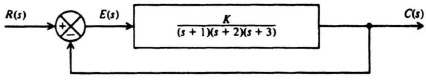
Figure P6.60
(a) The system has negative feedback.
(b) The system has positive feedback.
6.61. The transfer function of an unknown element in a control system can be determined by measuring its frequency response using a sinusoidal input. For a particular element, the frequency and amplitude data shown in Table P6.61 were obtained.
The form of the transfer function is given by
![]()
Determine the values of K, ωa, ωb, and ωc.
Table P6.61. Experimental Data
| ω | G(jω) in dB |
| 0.1 | 66 |
| 0.2 | 60 |
| 0.4 | 54 |
| 0.7 | 51 |
| 1.0 | 49 |
| 2.0 | 47 |
| 4.0 | 46 |
| 7.0 | 45 |
| 10.0 | 43 |
| 20.0 | 39 |
| 40.0 | 34 |
| 70.0 | 28 |
| 100.0 | 23 |
| 200.0 | 13 |
| 400.0 | 2 |
| 700.0 | −8 |
| 1000.0 | −14 |
6.62. The transfer function of an element used in a feedback system is not known explicitly, but its frequency response has been measured experimentally and is given in Figure P6.62. Based on your knowledge of Bode-diagram characteristics, determine the transfer function of this element.
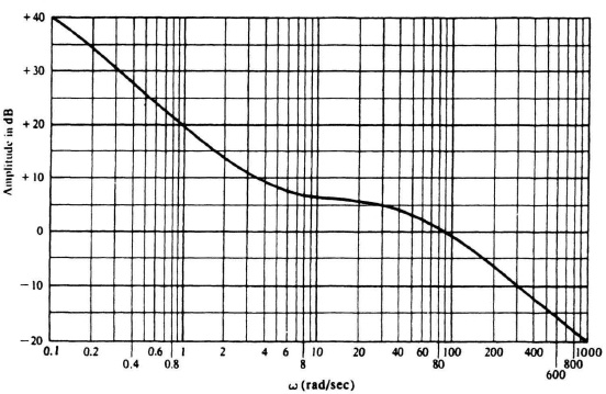
Figure P6.62
6.63. Electromechanical nose-wheel steering systems have been developed that can supply general aviation short-haul aircraft with needed maneuverability and durability [55]. These intermediate-sized aircraft must be able to utilize small airfields, many of which do not have elaborate service and maintenance facilities. During takeoff from such landing strips, the task of keeping the aircraft on the proper heading is achieved by utilizing nose-wheel power steering provided by this device. The block diagram of a nose-wheel steering system is illustrated in Figure P6.63. Pilot command signals are compared with a feedback signal representing the nose wheel’s heading. The resulting error signal is amplified and applied to a magnetic particle clutch, which activates the rotation of the wheel heading. Assuming that L/R = 0.1, Kc = 1, J = 1, Cv = 9, and Ke = 9, utilize the Bode diagram to determine the gain required to achieve a phase margin of 40°.

Figure P6.63
6.64. The proper design of man-machine control systems requires as much knowledge of the human element as that of the machine. Therefore, the determination of the human transfer function is very essential in order that the performance of man-machine systems can be evaluated. This problem can be better understood by referring to Figure P6.64, which depicts the classical compensatory manual tracking problem. In this configuration, an operator attempts to maintain a moveable follower coincident with a stationary reference point that represents the target. A very general and useful form of the human transfer function, GH(s), which can be applied to manual tracking problems, was provided in Problem 3.33. It is given by

Figure P6.64
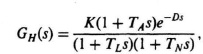
where D represents the operator’s transportation lag, TA represents the operator’s anticipation time constant, TL represents the operator’s error-smoothing lag-time constant, and TN represents the operator’s short neuro-muscular delay. Representative values for the elements are as follows [54]:
D = 0.2 sec ± 20%.
TA = 0-2.5 sec (variable),
TL = 0-20 sec (variable),
TN = 0.1 sec ±20%,
K = 1-100 (variable).
The gain K and the time constants TA and TL are considered to be variable according to the control task being performed. This transfer function has met with reasonable success for predicting manual tracking control system response where the bandwidth is relatively low. For this problem, assume that the human transfer function is given by the following expression:
![]()
Assume that the controlled system has a transfer function given by
![]()
Draw the Bode diagram and determine the phase and gain margin of the resulting system.
6.65. The pitch attitude control system for a booster rocket containing attitude and rate gyros is shown in Figure P6.65. Sketch the root locus and determine the maximum value of K that would permit stable operation.
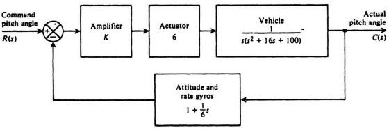
Figure P6.65
6.66. A unity feedback control system has the following forward transfer function:
![]()
(a) If the gain is set at 1.1 and one of the closed-loop poles is known to be located at s1 = −0.5, is the system stable?
(b) If the gain is increased to 30 and one of the closed-loop poles is known to be located at s1 = −6, is the system stable?
6.67. The root locus method can be used to study the stability of a motorcycle and rider combination. Analysis of a motorcycle/rider system must include a model of the rider in addition to the handling characteristics of the motorcycle. For this analysis, the approximate human model to be used for the system shown in Figure P6.67 is [54]:
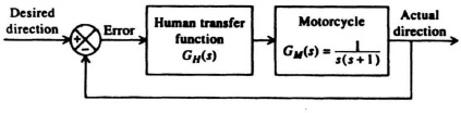
Figure P6.67
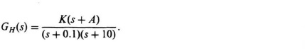
(a) Draw the root locus of this motorcycle/rider system assuming that the rider is new, his anticipation is very small, and therefore the “zero” term (s + A) can be neglected in the numerator of GH(s). Show all pertinent values on the root locus including the allowable range of K for stability.
(b) Draw the root locus of this motorcycle/rider system assuming that the rider has gained experience, and the anticipation term is finite. Assume that A = 1. Show all pertinent values on the root locus including the allowable range of K for stability.
(c) What conclusions can you reach by comparing the allowable range of gain for stability in parts (a) and (b)?
6.68. The roll attitude-control system for a missile containing attitude and rate gyros is shown in Figure P6.68.
(a) Sketch the root locus and indicate all pertinent characteristics.
(b) Find the maximum value of K that would permit stable operation.
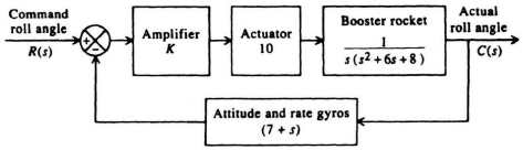
Figure P6.68
6.69. A block diagram of a unity negative-feedback positioning system used in a robot has a forward transfer function given by
![]()
(a) Sketch the root locus giving all pertinent characteristics of the locus. Identify all asymptotes, points of breakaway from the real axis, and the intersection of the root locus and the imaginary axis.
(b) At what value of gain does the system become unstable?
(c) When the system becomes unstable at the gain found in part (b), determine the location of all three roots of the system.
6.70. Consider the control system in Figure P6.70.
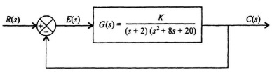
Figure P6.70
(a) Sketch the root locus of this control system. Determine all pertinent values on the root locus including the asymptotes, angles of departure, Kmax, and the crossing of the imaginary axis.
(b) We wish to operate this system at a gain which will result in the real part of all the closed-loop poles being equal. Determine the value of the gain and the real part of these closed-loop poles for this condition.
6.71. Determine the root locus for a negative-feedback system whose open-loop transfer function is given by

for 0 ![]() K
K ![]() ∞. (Hint: One of the points of breakaways from the real axis exists at −1.74). Indicate all pertinent points on the root locus, and determine the range of K for which the system is stable.
∞. (Hint: One of the points of breakaways from the real axis exists at −1.74). Indicate all pertinent points on the root locus, and determine the range of K for which the system is stable.
6.72. Repeat Problem 6.26 if we wish to design the control system for a phase margin of 45°.
6.73. Repeat Problem I6.9 for the following transfer function:
![]()