2.26.  STATE TRANSITION MATRIX

The state transition matrix relates the state of a system at t = t₀ to its state at a subsequent time t, when the input u(t) = 0. In order to define the state transition matrix of a system, let us consider the general form of the state equation [see Eq. 2.197]:

The Laplace transform of Eq. (2.252) is given by

where X(s) is the Laplace transform of x(t) and U(s) is the Laplace transform of u(t). Solving for X(s), we obtain

The inverse Laplace transform of Eq. (2.254) gives the state transition equation

Figure 2.37   Unit step response of system shown in Figure 2.29 obtained using the MATLAB Program in Table 2.12.

where the state transition matrix is defined by

The first term on the right-hand side of Eq. (2.255) is known as the homogeneous solution and is due only to the initial conditions; the second term on the right-hand side of Eq. (2.255), the convolution integral, is known as the particular solution and is due to the external forcing function. Equation (2.256) is defined as the state-transition matrix of the system for t0. When the input u = 0, Eq. (2.256), reduces to

The matrix Φ(t) is defined as the state transition matrix, because it relates the transition of the system state at time t₀ = 0⁺ to the state at some subsequent time t. It has the following properties:

Very often it is desired to use a more general initial time t₀. Equation (2.255) can be modified by letting t = t₀. Solving for x(0⁺), we obtain the following expression:

Using Eq. (2.261), Eq. 2.262 can be rewritten as

Substituting Eq. (2.263) into Eq. (2.255), the following expression is obtained:

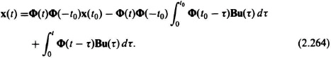
Using Eq. (2.259), Eq. (2.264) can be reduced to

Equation (2.265) is the solution of Eq. (2.252) for t t₀.

As an example of determining the state transition matrix, consider the open-loop system where the transfer function of the controlled process is given by

Its corresponding differential equation is given by (t) = u(t). Defining the state variables as

the system can be described by the following two first-order differential equations:

Therefore, the entire system can be described by the state equation

where

The state transition matrix, which is defined by

can be obtained from Eq. (2.270). We find

From Eq. (2.188), we know that

Therefore

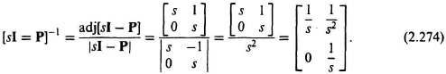
The state transition matrix defined by Eq. (2.256) is the inverse transform of this matrix. It is given by

With knowledge of the state transition matrix, we can easily determine the values of states x₁(t) and x₂(t) as a function of time. Let us assume that the initial values of the states are given by the following initial-state vector:

We can find the state vector x(t) as a function of time from Eq. (2.257) as follows:

Therefore, substituting Eqs. (2.275) and (2.276) into (2.277), we obtain

Solving for x₁(t) and x₂(t), we obtain the following:

These expressions are plotted in Figure 2.38.

The state transition matrix may also be derived from the state-variable diagram. As an example of the technique, consider a system described by the differential equation

Figure 2.38   Plot of states x₁(t) and x₂(t) as defined in Eqs. (2.279) and (2.280), respectively.

The Laplace transform of Eq. (2.281) yields

and dividing top and bottom by s², we obtain

Defining

Eq. (2.283) may be rewritten as

From Eq. (2.285) and the relation

the state-variable diagram for this system is obtained as illustrated in Figure 2.39. In addition, for generality, it is assumed that the states of the system, x₁(t) and x₂(t), have the initial conditions x₁(0) and x₂(0), respectively, at the inputs to each integrator. The corresponding state-variable signal-flow graph is given by Figure 2.40. The resulting transformed state equations of the system are obtained from this state-variable signal-flow graph using Mason’s formula [Eq. 2.135]:

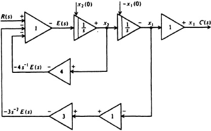
Figure 2.39   State-variable diagram for system where C(s)/R(s) = 1/(s² + 4s + 3).

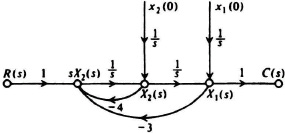
Figure 2.40   State-variable signal-flow graph corresponding to the state-variable diagram of Figure 2.39.

where

Simplifying Eqs. (2.287)–(2.289), we obtain the following pair of equations:

These two equations can be put into the following form:

From Eq. (2.292), we can obtain the state transition matrix by taking the inverse Laplace transform. It is assumed in the following solution that r(t) = U(t) and R(s) = 1/s:

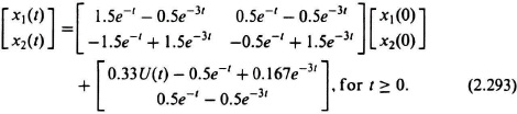
Therefore, the state transition matrix is given by

Once the state transition matrix is obtained, the evaluation of the time response is easily obtained.

This technique unfortunately shows that the use of the state-variable diagram and the state-variable signal-flow graph method for determining the state transition matrix is extremely inefficient compared with calculating it directly from Eq. (2.256). However, the method utilizing the state-variable diagram in conjunction with the signal-flow graph does have advantages in certain situations, because it offers other choices of state variables and permits application of Mason’s theorems for determining the relationships among the various states required in the state transition matrix.