4.6.  MODELING THE TRANSFER FUNCTIONS OF CONTROL SYSTEMS [2]

In the previous material presented, we designate transfer functions to various elements of the control system. For example in Figure 2.9, some of the elements shown in this block diagram are designated G₁(s), G₂(s), G₃(s), G₄(s), etc. How do we determine their actual transfer functions? If these elements are simple networks as described in Table 2.4, we can then use their corresponding theoretical transfer functions as shown in Table 2.4. If they are electromechanical motors, we can use the transfer functions for these devices that are derived in Section 3.4. However, in the case of motors and other devices, how do we know whether the actual transfer function agrees with the theoretical transfer function? What if we have an unknown device, or “black box,” and we do not know what its transfer function is at all?

To address this problem, we can apply a test signal to the device and measure its output. From knowledge of the input test signal and the measured output, we can then determine the device’s actual transfer function. The most commonly used test signals are a unit step and a sinusoidal signal. We use the unit step to obtain a transient response of the device. This approach is presented in this section. The frequency-response approach for testing the frequency reponse of a device to a sinusoidal input signal is presented in Chapter 6.

Suppose we have a linear control system consisting of only one element, G(s), as shown in Figure 2.7 and we do not know its transfer function. To determine its transfer function, we will apply a unit step input and measure the output’s transient response. Therefore, r(t) = U(t), and R(s) = 1/s. The possible transient responses for the outputs, c(t), are shown in Figure 4.2. How do we model this output transient response into a describable function for c(t)?

Having determined the function c(t), the procedure for finding G(s) would proceed as follows. The Laplace transfer function of c(t), C(s), is then determined. Since we know the Laplace transform of the unit step input is R(s) = 1/s, we can then determine the transfer function of G(s) as follows:

The resulting transient response may take on the characteristics of any of the results illustrated in Figure 4.2. For example, it may result in a critically damped, over-damped, or underdamped system.

Observe from the transient responses in Figure 4.2 that the various responses are smooth and monotonic. Let us assume that c(t) is given by the sum of exponential terms as follows:

where c_ss represents the final-value of c(t) as t approaches infinity. Simplifying Eq. (4.47) and focusing only on “−a” as the slowest or smallest root, we obtain the following:

Taking the logarithm to the base 10 of Eq. (4.48), we obtain the following:

Equation (4.50) is the equation of a straight line, We can fit a straight line to the plot of log₁₀[c(t) − c_ss], or log₁₀[c_ss − c(t)] if K₁ is negative, and we can estimage K₁ and a. Having estimated K₁ and a, we can then plot c(t) − c_ss − K₁e^−at which is determined by subtracting the line K₁e^−at from the original data. At this point, the curve is approximately K₂e^−bt and the plot represents log₁₀K₂ − 0.434bt. The process is repeated until the residual (error) in the modeling process approaches zero.

To illustrate this procedure, let us consider the transient data in Table 4.1 which represent the transient response of a closed-loop, second-order, control system given by the following transfer function

to a unit step input. The transient response is plotted in Figure 4.10 as the solid curve. The control system whose transfer function is given by Eq. (4.51) represents a critically damped control system whose two roots are equal and lie at −3.0 on the negative real axis. A plot of the absolute value of log₁₀[1 − c(t)] is illustrated in Figure 4.11. From the straight-line fit obtained using MATLAB, the vertical axis intercept is 0.3436. Therefore,

Figure 4.10   Transient response of the control system whose transfer function is given by Eq. (4.51) to a unit step input, and a model fit ĉ(t).

with the result that K₁ = −2.2057, and K₁ is negative because c_ss is greater than c(t). The slope of this straight line is −1.104. Therefore,

and a = 2.5430.

The next step is to subtract this line from the given data for c(t) and plot the log of this result. This is performed in Figure 4.12. The vertical intercept of this plot is 0. 6517. Therefore,

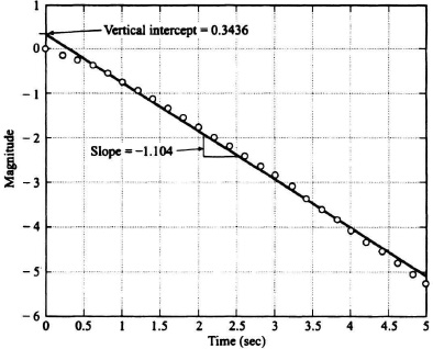
Figure 4.11   Straight-line fit to the absolute value of log₁₀[1 − c(t)].

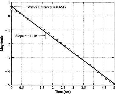
Figure 4.12   Straight-line fit to the subtraction of the straight-line obtained in Figure 4.11 from the given data for c(t).

with the result that K₂ = −4.4847, and K₂ is negative because c_ss is greater than c(t). The slope of this line is −1.106. Therefore,

and b = 2.5466. Combining the results of Eqs. (4.47), (4.52), (4.53), (4.54), and (4.55), we obtain the following estimate for ĉ(t):

Because we want c(0) = 0, we must adjust the estimate of Eq. (4.56) by adding the following term which is obtained from the steady-state value and the coefficients of K₁ and K₂:

Therefore, we add +2.8452 to the coefficients K₁ and K₂ and obtain the following estimate for c(t):

The result of this estimate from Eq. (4.58) is plotted in Figure 4.10 and superimposed on the result of the actual unit step response of c(t). This figure also illustrates the error between c(t) and the estimate to ĉ(t). Table 4.1 also contains the actual data for c(t), the estimated value for ĉ(t) and the error between c(t) and the estimated value of ĉ(t).

Therefore, the estimated or modeled transfer function can be obtained as illustrated in Eq. (4.46). Taking the Laplace transform of (4.58), we obtain the following:

Dividing Ĉ(s) from Eq. (4.59) by R(s) = 1/s, we obtain the following:

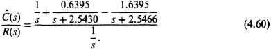
This can be simplified to the following result:

The resulting modeled value of Ĉ(s)/R(s) from Eq. (4.61) contains a zero term in the left half-plane, while the known transfer function of C(s)/R(s) in Eq. (4.51) does not contain a zero term.

The resulting estimated value of c(t) is fairly close to the actual value of c(t) as shown in Figure 4.10. This example illustrates that this procedure is very sensitive, and great care must be taken to ensure accuracy. Therefore, MATLAB was used in solving this example. If this procedure were done with hand calculations, a poorer fit would undoubtedly result. Another factor which must be brought to the attention of the reader is that noise can corrupt the results and lead to erroneous models. Therefore, in obtaining the test data, ensure that the data have a very good signal-to-noise ratio. More sophisticated and accurate modeling procedures can be found in Reference 2.