ANSWERS TO SELECTED
PROBLEMS

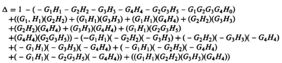
CHAPTER 1

1.1. An electrical signal proportional to the difference between the desired heading (gyroscopic setting) and original heading is amplified by the power amplifier. The amplified signal drives the motor which turns the rudder until the desired heading and actual heading of the ship are in agreement, and the corresponding electrical signal that is proportional to the difference between these two headings is zero. This is an open-loop control system as there is no feedback signal.

1.2. The rudder’s positioning can be made into a closed-loop control system by fastening a resistor to the rudder in a similar manner to the resistor that is fixed to the ship’s frame. An electrical feedback signal can then be obtained of the actual position, which can be appropriately compared with that of the desired, or reference, position.

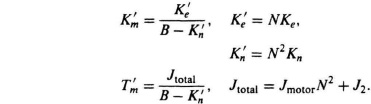
1.3. If the reference temperature of the thermostat is changed, the reference input to the control system changes, and an electrical error signal resuls. The electric hot-water heater will then change the temperature of the water until the difference between the reference input and actual temperatures is zero.

1.4. A change in the ambient temperature surrounding the tank manifests itself as a disturbance input within the heating control system. The explanation of the system’s resulting control action is similar to that discussed in the book for a disturbance occurring in an automatic speed-control system (see Figure 1.10).

1.6. The speed of an internal combustion engine can be varied by adjusting the spark setting and fuel-air mixture. By utilizing a tachometer to feed back an electrical signal proportional to the internal combusion engine’s speed and comparing it with a reference voltage that is proportional to the desired speed, the spark setting and fuel-air mixture can be theoretically adjusted to control the speed of the engine.

1.7. (a) The basic system would require that the elevator’s actuating signal be proportional to posiiton, velocity, and acceleration. Theoretically, this could be obtained by feeding back electrical signals proportional to position, velocity, and acceleration, and comparing these signals with reference signals representing the desired values. In practice, this can be simplified by placing integrators properly within the control system in order that only electrical signals proportional to position, and perhaps velocity, need be sensed.

(b)  Specifications must be placed on the velocity and acceleration capabilities in order that they be limited to safe values from the passenger’s viewpoint.

1.8. Assuming that safety brakes are not utilized in the feedback control system devised, the man entering the elevator acts as a disturbance force in the feedback control system. The functioning of the control system’s resulting action is similar to that discussed in Chapter 1 for a disturbance torque occuring in an automatic speed-control system (see Figure 1.10).

1.17. (Part 4) See Figure A1.17.

Figure A1.17

1.19. See Figure A1.19

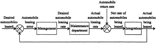
Figure A1.19

CHAPTER 2

2.2. v(t) = 2.5(1 − e^−6t)U(t).

2.5. (a)

(b)  

(c)  y(t) = (1.33 − 33.3e^−1.5t + 40e^−t)U(t).

2.8. The final-value theorem cannot be used for this function to determine its final value, because F(s) is not analytic in the right half-plane (pole exists at s = 2).

2.9. (a) f_A(t) = (−5te^−2t − 10e^−et − 0.0315e^−10.48t + 10.0315e^−1.52t)U(t),

(b)  

(c)  f_C(t) = (0.5 − 0.25e^−7.47t − 0.250e ^−0.53t)U(t).

2.13. Output of first system: −2e^−2tU(t).

Output of second system: (4e^−2t − 8te^−2t)U(t).

2.18.

2.20.

(a)

(b)

2.21.

(a)

(b)

2.25.

2.26.

2.28

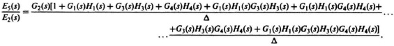
where (all parameters in Δ are a function of s):

2.35.

(a)  

(b)  

2.39. One possible solution to this problem is shown in Figure A2.39.

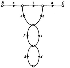
Figure A2.39

2.42. (a) Defining x₁(t) = c(t) and x₂(t) = (t), the plant dynamics become

(t) = x₂(t), (t) = 2x₂(t) − x₁(t),

or in the vector/matrix form

(t) = Px(t),   c(t) = Lx(t),

where

(b)  With x₁(t) = c(t) and x₂(t) = (t), the plant dynamics become

(t) = x₂(t), (t) = −2x₂(t) − x₁(t) + A,

or in vector/matrix form

(t) = Px(t) + Bu(t),   c(t) = Lx(t),

where

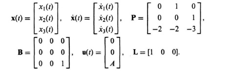
(c)  With x₁(t) = c(t), x₂(t) = (t), and x₃(t) = (t), the plant dynamics becomes

(t) = x₂(t),

(t) = x₃(t),

(t) = −2x₁(t) − 2x₂(t) − 3x₃(t),

or, in vector/matrix form,

(t) = Px(t),   c(t) = Lx(t),

where

(d)  With x₁(t) = c(t), x₂(t) = (t), and x₃(t) = (t), the plant dynamics becomes

(t) = x₂(t),

(t) = x₃(t),

(t) = −2x₁(t) − 2x₂(t) − 3x₃(t) + A,

or in vector/matrix form,

(t) = Px(t) + Bu(t),   c(t) = Lx(t),

where

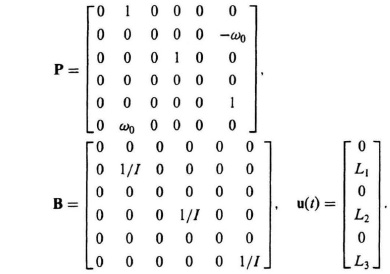
2.43. With x₁(t) = θ₁(t), x₂(t) = (t), x₃(t) = θ₂(t), x₄(t) = (t), x₅(t) = θ₃(t), and x₆(t) = (t), the plant dynamics become

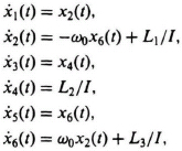
or in vector/matrix form

(t) = Px(t) + Bu(t),

where

2.45. With x₁(t) = v(t) and x₂(t) = (t), the plant dynamics become

2.47. The differential equation of the system is given by

(t) + 4(t) + c(t) = r(t).

With x₁(t) = c(t) and x₂(t) = (t), the plant dynamics become

(t) = x₂(t), (t)= − x₁(t) − 4x₂(t) + r(t),

or in vector/matrix form

(t) = Px(t) + Br(t),

where

2.61. With x₁(t) = c(t), x₂(t) = (t), and x₃(t) = (t) the state equations become

(t) = x₂(t),

(t) = x₃(t),

(t) = −400x₁(t) − 820x₂(t) − 412x₃(t) + 400r(t),

or in vector/matrix form

(t) = Px + Br(t),

where

The output equation is given by

c(t) = Lx(t),

where

L = [1  0  0].

2.64. Φ(t) =

2.75 (a)          

(b)  x₁(t) = 44,000 + 156,000e^−5t,
x₂(t) = 88,000 − 78,000e^−5t,

(c)       t = 0.334.

2.77. (a)

(b)   c(t) = −40e^−3t + 50e^−2t,  t ≥ 0
(t) = 120e^−3t − 100e^−2t,  t ≥ 0.

2.78. (a)         

(b)        

2.79.        

(b)        

CHAPTER 3

3.1. (a)

(b)         

3.2. (b)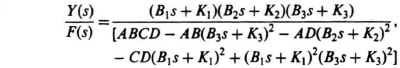         

where

A = M₁s² + B₁s + K₁,

B = M₂s² + (B₁ + B₂)s + (K₁ + K₂),

C = M₃s² + (B₂ + B₃)s + (K₂ + K₃),

D = M₄s² + B₃ + K₃.

3.3. (b)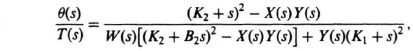          

where

W(s) = J₁s² + B₁s + K₁,

X(s) = J₂s² + (B₁ + B₂)s + (K₁ + K₂),

Y(s) = J₃s² + (B₂ + B₃)s + (K₂ + K₃).

3.4. (a)          

(b)         

3.5.          

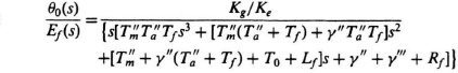
3.7. Defining the following terms

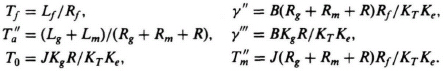
(a)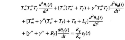          

(b)          

3.8. (b)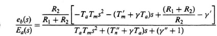         

where

3.11.

3.13.

3.14.          

where

3.15.         

3.21. (a) MR².

(b)  

(c)  

(d)          X(t) = Rθ₀(t).

(e)          

(f)          

3.22.          a_LA = 1.1111a_LB.

Therefore, we conclude that System A has the higher initial load acceleration.

3.24.          

3.27.          

CHAPTER 4

4.1. (a) ω_n= 47.3 rad/sec. ζ = 1.028.

(b)  Percent overshoot = 0, time to peak = ∞.

(c)  The error as a function of time can be plotted from the following expression:

e(t) = 2.62e^−37.2t − 1.63e^−60.2t,   t 0.

4.6 (a)

(b)  ω_n = 8 rad/sec, ζ = 0.5.

(c)  Maximum percent overshoot = 16.4%, time to peak = 0.452 sec.

4.11. K_a = 2.79.

4.13. (a) ω_n = 4.47 rad/sec.

(b)  Damping ratio = 0.37.

(c)  Maximum percent overshoot = 29%.

(d)  t_p = 0.76. sec.

4.14. (a) ω = 4.47 rad/sec.

(b)  Damping ratio = 0.56.

(c)  Maximum percent overshoot = 12%.

(d)  t_p = 0.85 sec.

4.16.
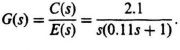
          K_m = 1.4591,
          T_m = 0.05457 sec.

4.19. (c) c(t) = 1 + 0.1314e^−1.9835t − 1.1314e^−1.9838t

CHAPTER 5

5.1. (a)

(b)  

(c)  

5.2. (a)          

(b)          

(c)          

(d)          

(e)          In the vicinity of

5.6.          

5.17. (a) 4.

(b)  Infinity.

5.20. (a)          

(b)          

5.24.          

5.26. (a) 1.

(b)  Infinity.

(c)  Add a second pure integration to G(s).

5.27. (a) Zero.

(b)  2.4.

(c)  Infinity.

5.30. (a) On the assumption that J_L ≫ J_mN²,

(b)  ω_n = 4.37 rad/sec; ζ = 10.3.

(c)  0%; ∞ sec.

(d)  Zero.

(e)  0.476.

(f)  Infinity.

5.38. K₁ = 0.112,     β₁ = 0.77,     β₂ = 4.36.

5.44. (a) e_ss = 0

(b)  e_ss = 0.1

(c)  K = 20

5.45. K_m = 0.255

CHAPTER 6

6.3. (a) s³ + s² + Ks + 4 = 0.

(b)  Range of K where the system is stable:

K > 4.

6.8. (a) Stable.

(b)  Unstable with two poles in right half-plane.

(c)  Stable.

(d)  Stable.

6.13. C + 0.3 − A > 0,   T − B + D > 0.

6.14. (a) Unstable with two poles in right half-plane.

(b)  Unstable with two poles in right half-plane.

(c)  Unstable with two poles in right half-plane.

(d)  Unstable with two poles in right half-plane.

6.18. System is unstable with two roots in the right half-plane.

6.19. (a) Unstable with two poles in right half-plane.

(b)  Unstable with two poles in right half-plane.

(c)  Stable.

6.25. (a) Pertinent characteristics of the Bode diagam are as follows:

1. Crossover frequency = 5.72 rad/sec.

2. Phase margin = −10.53°.

3. Gain margin = −4.44 dB.

(b)  Pertinent characteristics of the Bode diagram are as follows:

1. Crossover frequency = 0.7216 rad/sec.

2. Phase margin = −17.76°.

(c)  Pertinent characteristics of the Bode diagrams are as follows:

1. Crossover frequency = 2.935 rad/sec.

2. Phase margin = −24.73°.

3. Gain margin = −∞.

(d)  Pertinent characteristics of the Bode diagram are as follows:

1. Crossover frequency = 0.2792 rad/sec.

2. Phase margin = 16.24°.

3. Gain margin = ∞.

6.27.          

6.30. (a) Phase margin = 43.21°, gain margin = 15.56 dB.

(b)  Phase margin = 43.21°, gain margin = 15.56 dB.

(d)  K_p = ∞, K_v = 2, K_a = 0.

(e)  2.5 rad.

6.32. (b) Crossover frequency = 3.757 rad/sec, phase margin = −8.891°; gain margin = −3.098 dB, system is unstable.

(c)  K_p = ∞, K_v = 10, K_a = −0.

(d)  4 rad.

6.33. (b) K_a = 45.

(c)  Crossover frequency = 1.498 rad/sec, phase margin = −8.522°, gain margin = −∞; system is unstable.

6.34. (a) Crossover frequency = 4.483 rad/sec, phase margin = 32.44°, gain margin = 8.657 dB.

(b)  K = 9.9.

(c)  Crossover frequency = 13.61 rad/sec, phase margin = −30.62°, gain margin = −11.26 dB.

6.35. (c) ω_p = 3.742 rad/sec, M_p = 6.30 dB.

(d)  No.

6.36. (c) ω_p = 2.472 rad/sec, M_P = 1.304 dB.

(d)  No.

6.37. (a) The Bode diagram indicates a crossover frequency of 23.51 rad/sec and a phase margin of 20.61°.

(c)  ω_p = 23.46 rad/sec, M_p = 8.929 dB.

(d)  No.

6.42. (a) K = 1.91.

(b)  ω_p = 2.472 rad/sec, M_p = 1.304 dB.

6.43. (b) M_p = 5.283 dB, ω_p = 8.165 rad/sec.

6.44. (b) System is unstable.

6.45. (a) Pertinent characteristics of the root are as follows:

1. Root locus occurs along the real axis between the origin and −1, and between −10 and −∞.

2. The asymptotes intersect the real axis at −3.67 with angles of ±60°.

3. The point of breakaway of the root locus from the real axis occurs at −0.49.

(b)  K = 11.

6.46. (a) The root locus lies along the imaginary axis.

(b)  Pertinent characteristics of the root locus are as follows:

1. Root locus occurs along the real axis at the origin and between −1 and −10.

2. The asymptotes intersect the real axis at −4.5 with angles of ±90°.

3. The points of breakaway of the root locus from the real axis occur at 0, −2.5, and −4.

4. The root locus indicates that the system is stable.

(c)  Pertinent characteristics of the root locus are as follows:

1. Root locus occurs along the real axis between the origin and −1, and at −4.

2. The asymptotes intersect the real axis at −3.5 with angles of ±90°.

3. The root locus indicates that the system is stable for all values of gain.

(d)  Pertinent characteristics of the root locus are as follows:

1. Root locus occurs along the real axis at the origin, −0.1, and between −4 and −5.

2. The asymptotes interesect the real axis at −4.4 with angles of ±90°.

3. The points of breakaway of the root locus from the real axis occur at 0, −0.1, and −4.5.

4. The root locus indicates that the system is stable.

6.47. Pertinent characteristics of the root locus are as follows:

1. Root locus occurs along the real axis at the origin, between −0.01 and −0.1, and between −1.67 and −∞.

2. The point of breakaway of the root locus from the real axis occurs at 0 and −3.4.

3. The root locus crosses the imaginary axis at ±j0.386.

4. The root locus indicates that the system is stable for 0.14 < K < ∞.

6.68. (a) Pertinent characteristics of the root locus are as follows:

1. Root locus occurs along the real axis between the origin and −2, and between −4 and −7.

2. Asymptotes intersect the real axis at 0.5 with angles of ±90°.

3. The point of breakaway of the root locus from the real axis occurs at −0.92.

(b)  K_max = 4.8 at ±7.4833j.

6.71. Pertinent characteristics of the root locus are as follows:

1. Root locus occurs along the real axis between the origin and −3.125, and from −8 to −100.

2. Asymptotes intersect the real axis at −47.56 with angles of ±90°.

3. The points of breakaway of the root locus from the real axis occur at −1.74 and at −46.22; a point of break-in occurs at −15.58.

4. The root locus indicates that the system is stable.

6.72. K = 1.414

6.73. (a) Asymptotes are ±60° which intersect the real axis at −2. Root locus exists on the real axis from −2 to minus infinity.

(b)  K_max = 64, and the root locus intersects the imaginary axis at ±j3.46.

CHAPTER 7

7.1. (a) The electrical network illustrated in Table 2.4, items 3, with

R₁ = 690kΩ, R₂ = 51kΩ, C₁ = 1.38μF

and cascaded with an amplifier whose gain is 4.6 will satisfy the specifications

(b)  The electrical network illustrated in Table 2.4, item 4, with

R₁ = 690kΩ, R₂ = 51 kΩ, C₂ = 1.38μF

and cascaded with an amplifier whose gain is 4.6 will satisfy the specifications.

(c)  The electrical network illustrated in Table 2.4, item 5, with

R₁ = 595kΩ, R₂ = 25kΩ, C₁ = 1.68μF C₂ = 4μF

will satisfy the specifications.

7.2. (a) ζ = 0.5; ω_n = 4 rad/sec; maximum percent overshoot = 16.4%; steadystate error = 0.25.

(b)  b = 0.15.

(c)  Maximum percent overshoot = 1.5%; steady-state error = 0.4.

(d)  Add a high-pass filter in cascade with the tachometer as illustrated in Figure 7.15.

7.5. (a) G_c(s) = 1 + 0.382s.

(b)  b = 0.382.

7.7.

7.8. (a)

the attenuation of 1/178.6 due to the two lead networks is assumed to be compensated for by increasing the gain of the amplifier by 178.6. The result is a phase margin of 46.9° at a gain crossover frequency of 6.4 rad/sec, and a gain margin of 32.8 dB at a phase crossover frequency of 68 rad/sec.

(b)  

7.11. A phase-lead network whose transfer function is

The result is a phase margin of 61.8° at a gain crossover frequency of 0.49 rad/sec, and a gain margin of 22.4 dB at a phase crossover frequency of 3.08 rad/sec, assuming that the attenuation of the phase-lead network of is compensated for by boosting the gain of the amplifier by a factor of 15. Therefore, this phase-lead network achieves the design specification of a minimum phase margin of 60°.

7.12. Same answer as for Problem 7.11.

7.14. Two cascaded phase-lead networks are required to meet these specifications. Their transfer function, together with the gain found in Problem 6.34, is given by

The constant attenuation of 400 due to the characteristics of these two phase-lead networks must be made up by an amplification increase of 400. The resulting phase margin is 46.09° at a gain crossover frequency of 55.58 rad/sec.

7.15.

(a)  ω_c = 3 rad/sec.

(b)          

It is assumed that the attenuation of 1/40 is compensated for by increasing the gain of the amplifier. This phase-lead network provides a phase margin of 71.86° at a new gain crossover frequency of 8.078 radians/second.

7.20. (a)

The constant attenuation of 1.08 due to the characteristics of this phase-lead network must be made up by an amplification increase of 1.08.

(b)  For part (a), ω_p = 2.375 rad/sec, M_p = 1.154 dB.

7.21. (a)

The attenuation due to the phase-lead network is assumed to be compensated for by increasing the gain of the amplifiers.

(b)  For the phase-lead network, M_p = 0.7513 dB, ω_p = 3.864 rad/sec.

7.23. The phase-lag network is given by

7.27. (a) b = 0.25.

(b)  e_ss = 0.3024.

(c)  The transfer function of the rate feedback path is given by

(d)  e_ss = 0.0524.

7.28. K = 4.22.

7.38. K = 2.226

7.40. (a) K = 129.3.

(b)  M_p = 4.24 dB; ω_p = 10.67 rad/sec.

7.41 K = 25.57.

CHAPTER 8

8.2.

(a)   x₁(t) = −4x₁(t) − h₁x₁(t) + x₂(t)
x₂(t) = −Kx₁(t) + Kr(t)

(b)  s² + 4s + h₁s + K = 0.

(c)   h₁ = 10,
K = 48.

(d)   K₁ = 64,
K_p = 10.

(e)  The proportional plus integral controller configuration of part (d) produces a zero term which would aid in the stability compensation of this control system. The controller configuration of part (a) does not have this feature, and it would be more difficult to stabilize.

8.6. The synthesized system is illustrated in Figure A8.6, where

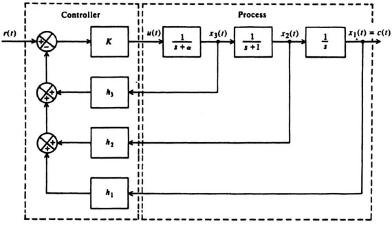
Figure A8.6

A root locus analysis indicates that a good choice of α is approximately 2.5. Therefore, h₃ becomes .

8.8. (a) Yes.

(b)  see Figure A8.8.

(c)   K = 20,000,
h₁ = 1,
h₂ = 0.00995.

(d)  Root locus shows that the system is stable.

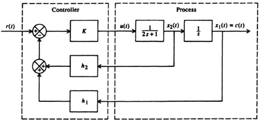
Figure A8.8

8.10. (a)

System is not controllable.

(b)  

System is observable.

8.11. (a)

System is controllable.

(b)  

System is unobservable.

8.13.

8.15.

8.17.

8.20.