6.1.  INTRODUCTION

For proper controlling action, a feedback system must be stable. Previous chapters have indicated that feedback systems have the serious disadvantage that they may inadvertently act as oscillators. A feedback control system must maintain stability when the system is subjected to commands at its input, extraneous inputs anywhere within the feedback loop, power-supply variations, and changes in the parameters of the elements comprising the feedback loop.

In the ensuing discussion, if a control system has zero initial conditions, then for every bounded input, the output is bounded and the system is stable. This is popularly referred to by control engineers as bounded input-bounded output (BIBO) stability. In this chapter, analysis is limited to linear time-invariant systems, that is, systems for which the principle of superposition is valid and which may be described by an ordinary linear differential equation with constant coefficients. The analysis of nonlinear systems is presented in Chapter 5, and digital control system stability is presented in Chapter 4 of the accompanying volume.

We showed in Section 4.4 that a control system’s total response was the sum of the forced response due to the external forcing function and the natural or homogeneous response due to the initial conditions. The analysis was performed for the second-order control system illustrated in Figure 4.7, and the resulting response to a unit-step input for this control system was given by Eq. (4.45).

Therefore, in general, the total response of a control system, c(t), is composed of the natural or homogeneous response due to the initial conditions, and the forced response due to the external input:

A linear, time-invariant control system is stable if the natural or homogeneous response approaches zero, and it is unstable if the natural or homogeneous response grows without bound as time approaches infinity. If the linear, time-invariant system neither grows nor decays, and an oscillation of constant magnitude results, which represents simple harmonic motion, then this is an indication of a marginally stable system. Such a system, however, is considered to be an unstable control system from a practical viewpoint.

Let us consider the stability of a linear, time invariant, control system which only has an input from its initial conditions, and then consider a control system which has a reference input, r(t). For the first case, we will assume that r(t) equals zero, and the control system is an nth-order system. Therefore, the output, c(t), can be expressed as follows:

where

and where g_k(t) represents the zero-input response due to c^(k)(0). Therefore, the control system is said to be zero-input stable if the zero-input response c(t) due to the finite initial conditions, c^(k)(0), approaches zero as t approaches infinity. The zero-input stability is also defined to be asymptotically stable because it is required that c(t) reaches zero as time approaches infinity. Linear, time-invariant, control systems which are BIBO, zero-input, stable, and asymptotically stable all require that the roots of the characteristic equation be located in the left half of the s-plane. Therefore, if a system is BIBO stable, then it must also be zero-input stable or asymptotically stable. Figure 6.1 illustrates the stable and unstable regions of the s-plane. Roots located on the imaginary axis result in a stable oscillation (e.g., simple harmonic motion), but this is considered to be an unstable s-plane condition to the practicing control-system engineer.

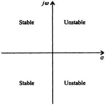
Figure 6.1   Stable and unstable regions of the s plane.

To illustrate the second case, where the linear time-invariant control system has a reference input, consider the following closed-loop transfer function of a control system which contains first-order real poles and zeros, and second-order quadratic poles:

Let the reference input be a unit step input. Therefore, R(s) = 1/s in Eq. (6.3), and expanding the resulting equation for C(s) into its partial fractions gives us the following:

where k_i is the residue of the pole at s = −p_i. Taking the inverse Laplace transform of Eq. (6.4), we obtain the following:

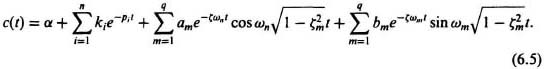
If all the closed-loop roots lie in the left half of the s-plane, then the exponential terms and the exponentially damped sinusoidal terms in Eq. (6.5) approach zero as time approaches infinity.

Therefore, it is necessary that the poles of the closed-loop transfer function must be in the left-hand part of the s-plane in order to obtain a bounded response. We can generalize this result as follows. A necessary and sufficient condition of control-system stability is that all its poles have negative real parts. A control system which has all its roots in the left-half plane is denoted as a stable system. If the control system does not have all the roots in the left-half plane, then the control system is denoted as being unstable. If the control system has roots on the imaginary axis, and all other roots are in the left-half plane, then the output response will have an oscillation of constant amplitude for a bounded input, and is denoted as being marginally stable. This case is considered to be unstable in practical control systems.

This chapter focuses attention on the stability of the general feedback system, which was illustrated in Figure 2.10. The closed-loop transfer function of this system, given by Eq. (2.121), is repeated below:

The characteristic equation for this generalized system can be obtained by setting the denominator of the system transfer function equal to zero:

In linear systems, stability is independent of the input excitation, and this is the equation that determines system stability. All the methods of stability analysis investigate this equation in some manner. One can show that if the roots of Eq. (6.7) lie in the left half-plane, the system is stable. However, the system is considered unstable if any of the roots of this equation have positive real parts or lie on the imaginary axis.

To illustrate this point, the transient response of the second-order system in Chapter 4 will be analyzed. Reconsider the underdamped case whose complex-conjugate poles lie in the left half of the complex plane, as shown in Figure 4.3. For that case, the transient response to a unit step input was shown to be an exponentially damped sinusoid in Figure 4.4. If the complex-conjugate poles of the second-order system were in the right half-plane, the transient response would be an exponentially increasing sinusoid and the system would be unstable. For the case of complex-conjugate poles that lie on the imaginary axis, the response would be a sinusoidal oscillation of fixed amplitude (simple harmonic motion). From a practical viewpoint, this would be considered to be unstable, also. These three cases are illustrated and compared in Figure 6.2 for three second-order systems labeled S1, S2, and S3 whose transfer functions and roots are given as follows:

(a)    S1:                    

Complex-conjugate roots are located at −0.2 ± 0.9798j.

(b)    S2:                    

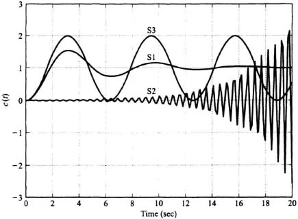
Figure 6.2   Unit step response of three second-order systems (S1, S2, S3)

Complex-conjugate roots are located at 0.3 ± 12.2438j.

(c)    S3:                    

Complex-conjugate roots are located on the imaginary axis at ±j.

Therefore, the system S1 has an exponentially decaying sinusoid and is stable; system S2 has an exponentially increasing sinusoid and is unstable; system S3 oscillates at a fixed amplitude and is unstable from a practical viewpoint.

In general, the following three approaches exist for determining stability:

1. Calculating the exact roots of Eq. (6.7)
2. Determination of the region of system parameters which guarantees that the roots of Eq. (6.7) have negative real parts.
3. State-variable method.

Using the first approach, the control engineer has at his or her disposal the following two methods:

(a)  Direct-solution utilizing the classical approach

(b)  Root-locus method

Using the second approach, the control engineer has at his or her disposal the following criteria:

(a)  Routh–Hurwitz criterion

(b)  Nyquist criterion.

Clearly, calculation of the exact roots using the classical approach can be extremely tedious. Usually, the designer is interested in the root-locus method and the criteria of the second and third approaches. This chapter represents each of these methods, except the classical approach, together with their relative merits. Additional graphical approaches based on the Nyquist criterion are also discussed. These include the use of the Bode diagram and Nichols chart. The state-variable approach permits the determination of the characteristic equation directly from knowledge of the state equations, and is illustrated in the following section. Application of these methods to actual design problems is deferred to Chapters 7 and 8.