PROBLEMS

7.1. Determine the circuit structure, the values of resistance and capitance, the gains of any amplifiers required, and the complex-plane plot for first-order networks having the following characteristics:

(a)  Phase lead of 60° at ω = 4 rad/sec, a minimum input impedance of 50,000 Ω, and an attentuation of 10 dB at dc.

(b)  Phase lag of 60° at ω = 4 rad/sec, a minimum input impedance of 50,000 Ω, and a high-frequency attenuation of 10 dB.

(c)  A phase-lag-lead network having an attenuation of 10 dB for a frequency range of ω = 1 to ω = 10 rad/sec and an input impedance of 50,000 Ω.

In all cases, limit the maximum values of resistance to 1 MΩ and capitance to 10 μF. Furthermore, assume that the loads on the networks have essentially infinite impedance.

7.2. The system illustrated in Figure P7.2 consists of a unity-feedback loop containing a minor-rate-feedback loop.

Figure P7.2

(a)  Without any rate feedback (b = 0), determine the damping ratio, undamped natural frequency, peak overshoot of the system to a unit step input, and the steady-state error resulting from a unit ramp input.

(b)  Determine the rate-feedback constant b which will increase the equivalent damping ratio of the system to 0.8.

(c)  With rate feedback and a damping ratio of 0.8, determine the maximum percent overshoot of the system to a unit step input and the steady-state error resulting from a unit ramp input.

(d)  Illustrate how the resulting steady-state error of the system with rate feedback to ramp inputs can be reduced to the same level if rate feedback were not used, and still maintain a damping factor of 0.8.

7.3. Repeat Problem 7.2 for the forward transfer function of the system given by 20/s(1 + s).

7.4. Figure P7.4 illustrates the block diagram of a roll control system used to limit the roll rate excursions of a missile by providing sufficient dynamic reaction to disturbing moments [12]. The disturbance moments result from changes in bank angle and steering control deflections. The basic limitation which determines the effectiveness of the roll-control system is the response of the aileron servo.

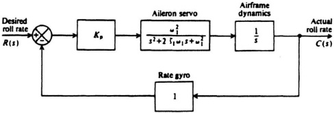
Figure P7.4

(a)  Determine the transfer function, C(s)/R(s), of the system illustrated in Figure P7.4.

(b)  Because the transient response is governed by a pair of dominant complex-conjugate poles, specify the requirements of the aileron servo parameters in order that the equivalent damping ratio of the system is approximately 0.5, and the equivalent undamped natural frequency of the system is approximately 4 rad/sec.

7.5. A unity-feedback system has a forward transfer function given by

It is desired to compensate this system so that the resulting damping ratio is unity (critically damped).

(a)  Using the classical approach, determine the time constant of a cascaded phase-lead network, containing a zero factor only, that can achieve this.

(b)  Using the classical approach, determine the rate-feedback constant of a minor rate-feedback loop which can achieve critical damping.

7.6. Repeat Problem 7.5 for the forward transfer function of the system given by

7.7. A phase-lag–lead network, whose general transfer function is given by Eq. (7.9), and whose gain and phase characteristics are illustrated in Figure 7.13, provides a phase lag at low frequencies and a phase lead at high frequencies. For the following phase-lag–lead network,

Find the frequency ω₀ where the phase angle of G(jω) becomes zero. For frequencies less than ω₀, this network acts as a phase-lag network; for frequencies greater than ω₀, this network acts as a phase-lead network.

7.8. It is desired that the system considered in Problem 6.32 have a minimum phase margin of 45° and a minimum gain margin of 20 dB. Cascade compensation is to be employed.

(a)  Specify the time constant of a phase-lead network (or networks) that can achieve this.

(b)  Repeat part (a) for a phase-lag network.

7.9. It is desired that the system considered in Problem 6.24 have a phase margin of 60° and a gain margin of 60 dB. Cascade compensation is to be employed. Determine the time constant of a phase-lag network (or networks) that can achieve this.

7.10. The temperature-control loop of a nuclear power plant is illustrated in Figure P7.10. The transfer function of the nuclear reactor can be adequately represented by

A time delay (or transportation lag) is included in this transfer function to account for the time required to transport the fluid from the reactor to the measurement point. A proportional-plus-integral (PI) controller is used for compensation.

Figure P7.10

Using the Bode diagram, determine the values of K₁ and K₂ in order to achieve a phase margin of 30° and a gain margin of 4 dB.

7.11. It is desired that the system considered in Problem 6.28 have a phase margin of 45° at the crossover frequency. Determine the stabilizing element required to achieve this.

7.12. It is desired that the system considered in Problem 6.33 have a phase margin of 45° at the crossover frequency. Determine the stabilizing element required to achieve this.

7.13. The H.S. Denison, shown in Figure P7.13a, the first large hydrofoil seacraft built and operated in the United States [13] was designed and built by the Grumman Aerospace Corporation for the Maritime Administration of the U.S. Department of Commerce. The 80-ton hydrofoil is capable of operating at speeds of 60 knots in seas containing waves nine feet high. A simplified schematic of the automatic control system of the H.S. Denison is illustrated in Figure P7.13b. It consists of transducers for sensing craft motions and a computer for transmitting commands to the electrohydraulic actuators [13]. Heave rate is fed symmetrically to the forward flaps; roll and roll rate are fed differentially to the forward flaps; pitch rate is fed to the stern foil. The stabilization control system maintains level flight by means of two main surface piercing foils located ahead of the center of gravity and an all-movable submerged foil aft. An equivalent block diagram of the pitch-control system is illustrated in Figure 7.13c. It is desired that the craft maintain a constant level of travel despite a wave disturbance U(s) whose energy is concentrated at 1 rad/sec. Assume that the specifications require that the pitch loop maintain a gain of 40 dB at 1 rad/sec in order to minimize the wave disturbance, and a crossover of 10 rad/sec for adequate response time. In addition, it is desired to have a phase margin of at least 50° at the gain crossover frequency of 10 rad/sec and a gain margin of 12 dB. Select the amplifier gain K_a and compensation network G_c(s) in order to achieve these requirements.

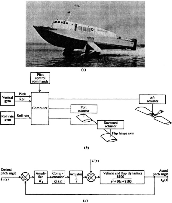
Figure P7.13   (a) Photograph of H. S. Denison. (Courtesy of Grumman Aerospace Corporation) (b) The automatic control system. (c) Block diagram of the pitch-control system.

7.14. It is desired that the system considered in Problem 6.34 have a phase margin of 45° at the gain crossover frequency. To achieve this, one or more phase-lead networks are introduced into the controller. Determine the compensation required and the resulting new crossover frequency to meet this specification.

7.15. A unity-feedback control system has a forward transfer function given by

(a)  Determine the gain crossover frequency and the phase margin of this control system.

(b)  A phase-lead network, as defined in Eq. (7.6), is to be added in cascade with G₀(s) so that the phase margin is 70°. Determine the phase-lead network which will achieve this phase margin.

7.16. A remotely piloted aircraft (RPA) for reconnaissance purposes over heavily defended terrain is to be controlled from a ground station. Use of the RPA will eliminate loss of human life if the aircraft is destroyed due to enemy action. The conceptual diagram of the RPA system is illustrated in Figure P7.16a.

An equivalent block diagram of the pitch attitude axis of the RPA system is illustrated in Figure P7.16b.

The transportation lag T₁ represents the delay caused by the man-in-the-loop at the ground station and the time it takes to transmit the signal from the ground station to the RPA. The transportation lag T₂ represents the time it takes for the return signal to be received by the ground station from the RPA. Assume that T₁ = 0.3 sec and that T₂ = 0.05 sec.

(a)  Determine analytically the gain crossover frequency needed to achieve a phase margin of 50°.

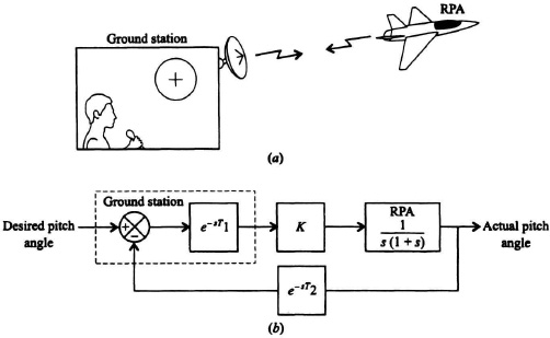
Figure P7.16

(b)  Without drawing a Bode diagram, determine the value of K needed to obtain the gain crossover frequency obtained in part (a).

7.17. Space vehicles, such as the space shuttle, using wings to maneuver while reentering the Earth’s atmosphere present an interesting control problem. Figure P7.17a illustrates a conceptual design of such a system and Figure P7.17b indicates the block diagram of the pitch-rate control of such a system [14].

Figure P7.17

(a)  Draw the Bode diagram of this system with K₁ = 1 and K₂ = 0. What are the resulting gain and phase margins?

(b)  Select the values of K₁ and K₂ which will result in a gain crossover frequency of 1 rad/sec, a phase margin of at least 30° and a gain margin of at least 16 dB.

7.18. It is desired that the system considered in Problem 6.31 have a phase margin of 55° at the crossover frequency, and a gain margin of 25 dB. In order to achieve this, two phase-lead networks are introduced into the controller. This results in the controller having a transfer function given by

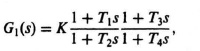
where K is the value of gain found in part (b) of Problem 6.31. Determine T₁, T₂, T₃, T₄, and the resulting new crossover frequency to meet this specification.

7.19. The design of the Lunar Excursion Module (LEM) shown in Figure P7.19a, was an extremely interesting problem [15]. The control, guidance, and navigation for the LEM are provided by an all-digital system from the sensors to the gas-jet propulsion units. For purposes of this analysis, the vehicle dynamics can be approximated by a double integration, as indicated in Figure P7.19b, which illustrates one axis of the attitude-control system. In addition, the torque T(s) is assumed to be proportional to the control signal U(s). Assume that J = 0.25 and

T(s) = 2U(s).

Utilizing the Bode diagram for solution, determine a lead-compensation network G_c(s) which will result in a crossover frequency of 5.1 rad/sec and a phase margin of 60°.

7.20. It is desired to add cascade compensation to the system considered in Problem 6.36 in order that the peak overshoot to a step input be approximately 12%.

(a)  Using the Nichols chart, design a phase-lead network which can achieve this.

(b)  With the compensation network chosen in part (a), determine the closed-loop amplitude and phase-frequency response.

7.21. It is desired to add cascade compensation to the system considered in Problem 6.42 in order that M_p = 0.75 while the same steady-state error is maintained.

(a)  Design a phase-lead network to achieve this.

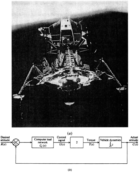
Figure P7.19

(b)  With the compensation network chosen in part (a), determine the closed-loop amplitude and phase frequency response.

7.22. It is desired that the system considered in Problem 7.21 have a peak overshoot of approximately 15% to a step input.

(a)  Utilizing a minor rate-feedback loop, specify the tachometer constant which can achieve this.

(b)  What will be the resulting system steady-state error to a unit ramp input with the minor rate-feedback loop added?

(c)  Utilizing a simple high-pass RC filter in cascade with the tachometer, determine the time constant of the network and the tachometer constant which will result in a 15% overshoot to a step input.

(d)  What will be the steady-state error to a unit ramp when the high-pass filter is cascaded with the tachometer?

7.23. It is desired that the system considered in Problem 6.45 have a damping ratio of 0.75 for the dominant complex roots. Using the root-locus method, determine the increase in gain and phase-lag network (s + nα)/(s + α) which can achieve this. Assume K_v = 15.

7.24. A unity-feedback control system has a forward transfer function given by:

(a)  Draw the Bode diagram of this control system and determine the resulting phase margin and gain margin.

(b)  To achieve an acceptable transient response for this system, the phase margin should be approximately 30° and the gain margin 20 dB. In addition, a sinusoidal disturbance is present at 0.1 rad/sec, and a gain of 60 dB is required at this frequency to nullify its effect. Design a passive compensation network which will achieve the desired transient response and accuracy, and also minimize the noise susceptibility of the system.

7.25. The block diagram of one axis of a robotic positioning system that uses rate feedback for compensation is illustrated in Figure P7.25.

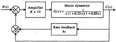
Figure P7.25

(a)  Without any rate feedback (b = 0), determine the gain crossover frequency, phase margin and gain margin of the uncompensated system using the Bode-diagram method.

(b)  For proper operation of the robot, a minimum phase margin of 65° and a minimum gain margin of 90 dB are desired. Using the Bode diagram, determine the amount of rate-feedback constant b which will achieve these requirements.

7.26. The system shown in Figure P7.26 contains a proportional plus integral (PI) controller. The PI controller contains a zero term at s = −K and a pole at s = 0. Therefore, the PI controller has infinite gain at zero frequency, and it behaves as a phase-lag network. This feature improves the steady-state characteristics.

Figure P7.26

(a)  Determine the steady-state error of this system to a unit step input.

(b)  Determine the steady-state error of this system to a unit ramp input.

(c)  Determine the range of gain K for which this system is stable.

7.27. A negative-feedback system containing unity feedback has a forward transfer function given by

The zero factor (s + A) in the numerator of this transfer is to be used to compensate the system. Utilizing the root locus, analyze the effects on system stability of the following values of A:

(a)  A = 1,     (b) A = 2,      (c) A = 3,
(d) A = 4,     (e) A = 6.

What conclusions can you draw from your results on the best value of A for compensating this system? What happens if A is greater than 6?

7.28. A unity-feedback control system has a forward transfer function given by:

We wish to use a proportional plus integral (PI) controller in cascade with G₀(s) to compensate this control system. The transfer function of this compensator is given by:

Select K so that the pair of dominant closed-loop poles for this control system is located at s = −0.5 ± 0.5j.

7.29. A unity-feedback control system has the following forward transfer function:

Determine the values of α so that the root locus will have zero breakaway points, not including the one at s equal zero.

7.30. The forward transfer function of a unity-feedback control system is given by the following:

(a)  Construct the root-locus digram for 0 ≤ K ≤ ∞, and show all pertinent values on the root locus. What conclusions can you reach from this root-locus diagram?

(b)  The system will be stabilized by mean of a rate-feedback element (e.g., tachometer) added in parallel to the unity feedback so that the total feedback transfer function becomes:

H(s) = 1 + s.

Construct the root locus of this compensated control system for 0 ≤ K ≤ ∞, and show all pertinent values on the root locus.

7.31. The transfer functions of a negative feedback system are given by the following:

(a)  Sketch the root locus.

(b)  Determine C(s)/R(s), with the denominator in factored form, if a damping ratio of 0.5 is required for the dominant roots.

7.32. Determine the increase in gain and phase-lag network compensation required to stabilize a unity-feedback system whose forward transfer function is given by

The requirement for the system damping ratio is 0.707, and the velocity constant is 100/sec.

7.33. A unity-feedback control system has a forward transfer function given by

It is desired that the system have a velocity constant of 15 and a damping ratio of 0.75. Using the root-locus method, determine the increase in gain and phase-lag network (s + nα)/(s + α) which can achieve this, assuming that the transient response is governed by a pair of dominant complex-conjugate poles.

7.34. A unity-feedback control system has a forward transfer function given by

It is desired that the system have a velocity constant of 150 and a damping ratio of 0.75. Using the root-locus method, determine the increase in gain and phase-lag network, represented by (s + na)/(s + a), which can achieve this. Assume that the transient response is governed by a pair of dominant complex-conjugate poles. Show all pertinent Points on the root locus before and after compensation.

7.35. The block diagram of a positioning system is shown in Figure P7.35.

Figure P7.35

(a)  Without any compensation, G_c(s) = 1, draw the root locus of the uncompensated system. On this diagram determine and show the following clearly:

•  Point (s) of breakaway from the real axis

•  Crossing (s) of the imaginary axis

•  K_max

•  All asymptotes.

(b)  It is desired that the system have a velocity constant of 4 and a damping ratio of 0.707. Using the root-locus method, determine the compensation G_c(s) which can achieve this. Assume that the transient response is governed by a pair of dominant complex-conjugate poles. Show all pertinent changes and Points on the root locus after compensation. (An exact recalculation of the point (s) of breakaway, the crossing of the imaginary axis, and K_max are not necessary.)

7.36. In order to obtain a control system which has an infinite velocity constant, a control-system engineer designs the control system of Figure P7.36, which he or she recognizes will need some compensation network, G_c(s).

Figure P7.36

(a)  Without any compensation, G_c(s) = 1, draw the root locus of this control system. From a practical viewpoint, is it stable?

(b)  The control-system engineer desires to use a passive compensation network for G_c(s), either a phase-lag or a phase-lead network. Assume that the resistors and capacitors that are available can provide a zero at −1 and a pole at −2, or a pole at −1 and a zero at −2. As the control-system engineer, which would you select and why? Draw the root locus for your stabilized control system (with either a phase-lag or a phase-lead network). Show all pertinent Points on your root locus.

7.37. The signal-flow graph of the temperature-control loop for a xylene chemical process [16] is shown in Figure P7.37. The temperature of the process, C(s), is related to the heat supplied to the process by the quadratic transfer function G_p(s). Temperature is measured by a sensor having a pole at s = −0.3, and the output of the sensor in the form of air pressure is compared with the desired value of temperature as indicated by the reference pressure R(s). The pressure difference (a measure of temperature error) actuates a pneumatic controller which provides as its output a pneumatic actuating signal applied to a steam valve. The valve, in turn, controls the flow of heat to the xylene column in order to minimize the error.

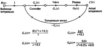
Figure P7.37

(a)  Draw the root locus for this system.

(b)  Determine the required gain K for a damping ratio of 0.5.

7.38. It is desired that the system considered in Problem 6.46 (b) have a damping ratio of 0.75 for the dominant complex roots. Using the root-locus method, determine the value of K which can achieve this.

7.39. A turbine speed-control system is illustrated in Figure P7.39. Assume that the transfer function of the control valve, turbine, and speed converter are as follows:

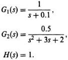
Figure P7.39

Assuming that the transient response is governed by a pair of dominant complex-conjugate poles, determine the value of the controller gain K in order that the system has a damping ratio of 0.5.

7.40. It is desired that the system considered in Problem 6.46 (c) have a damping ratio of 0.75 for the dominant complex roots. Using the root-locus method:

(a)  Determine the value of K which can achieve this.

(b)  Determine the values of ωp and M_p for the value of K found in part (s) using the Nichols chart.

7.41. Determine the gain needed for the system considered in Problem 6.46 (d) which can achieve a damping ratio of 0.75.

7.42. Unlike fixed-wing aircraft, which possess a moderate degree of inherent stability, the helicopter is very unstable and requires the use of feedback loops for stabilization. A typical control system involves the use of an inner automatic stabilization loop and an outer loop which is controlled by the pilot, who inserts commands into it based on attitude errors displayed to the pilot. Figure P7.42 illustrates the pitch-control system used on the S-55 helicopter [17]. When the pilot is not utilizing the control stick, the switch S₁ is open, which disengages the pilot control loop. The model of the pilot’s transfer function, G₁(s), includes a gain factor, an anticipation time constant of 1 sec, and an error-smoothing time constant of 10 sec [17].

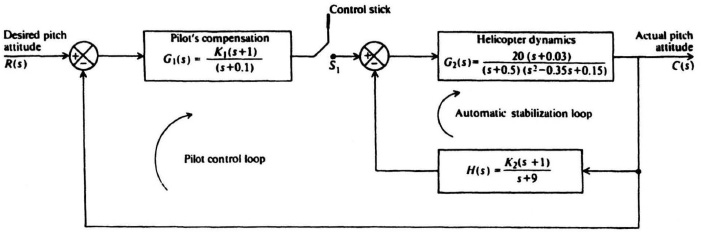
Figure P7.42

Figure P7.43

(a)  With the pilot control loop open, plot the root locus for the automatic stabilization loop and determine the gain K₂ which results in a damping ratio of 0.5 for the dominant complex roots.

(b)  Draw the root locus of the pilot control loop with K₂ set at the value determined in part (a). Determine the value of the pilot’s gain compensation factor K₁ in order that the pilot control loop have a damping ratio of 0.5.

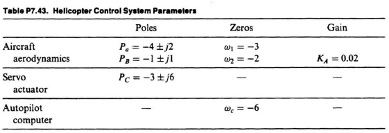
7.43. Many modern control systems are designed to be adaptive, in order that they can achieve a desired response in the presence of extreme changes in the system parameters and major external disturbances. Adaptive control systems are usually characterized by devices that automatically measure the dynamics of the controlled system and by other devices that automatically adjust the characteristics of the controlled elements based on a comparison of the measurements with some optimum figure of merit. Figure P7.43 illustrates an adaptive pitch flight control system [18]. It attempts to measure the exact location of a pair of dominant, variable, servo actuator poles that move in the complex plane, as a function of the flight conditions. The adaptive feature overcomes this problem by adjusting the gain in order to keep the location of these sensitive poles fixed in the complex plane. A test impulse train is injected into the system when the error is small. The performance computer determines the transient response of the system and compares it with an optimum desired response that is set at 2 half cycles of a transient response over a 3-sec interval of time. The performance computer is designed so that a count less than 2 over a 3-sec period will cause the adaptor motor to increase K, and a count greater than 2 over a 3-sec period will cause the adaptor motor to decrease K. Assume that the poles and zeros of the system are located in the complex plane as follows:

(a)  Draw the root locus of this system.

(b)  Determine the variable gain K that will result in a damping ratio of 0.3, assuming that the transient response is governed by a pair of dominant complex-conjugate poles.

7.44. Repeat Problem 7.33 for