2.28.  EVALUATION OF THE STATE TRANSITION MATRIX FROM AN EXPONENTIAL SERIES

The state transition matrix may be evaluated from an exponential series. Several methods have been proposed for its numerical evaluation. References [20] and [21] discuss one type of computational algorithm developed by Faddeev and Faddeeva for accomplishing this. However, this approach requires the Laplace-transform inversion of Φ(s). Unfortunately, this approach is very tedious for matrices of any size. This section presents a straightforward method that evaluates the state transition matrix based on its infinite matrix series definition [22]. Direct application of the series definition gives a very efficient and fast method that depends only on matrix multiplication. It is based on assuming a solution to the homogeneous state equation, as is commonly done in the classical method of solving linear differential equations.

In order to derive the exponential series definition of the state transition matrix [23], let us assume that the solution to the homogeneous state equation

is given by

where

and

We shall now work backwards (as in the classical method of solving differential equations) and prove that Eq. (2.316) is indeed the correct solution to Eq. (2.315). Following this procedure, the value of (t) is given by

A comparison of Eqs. (2.318) and (2.319) indicates that

Therefore, from the definition of Eq. (2.317), we find that

so that

or

is indeed a correct solution to Eq. (2.315).

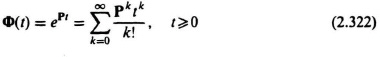
From this derivation, we can now extend our original definition of the state transition matrix (see Eq. 2.256) to the following:

Because the matrix series is uniformly convergent for any finite interval, the state transition matrix can be determined within prescribed accuracy using only a finite number of terms [5].

Let us apply this series solution approach for obtaining the state transition matrix to the same problem we solved in Section 2.26 from the definition of the state transition matrix provided in Eq. (2.256). The problem solved in Section 2.26 had the companion P matrix given in Eq. (2.270) as:

Substituting this value of P into Eq. (2.323), where k = 2 in this problem, we obtain the following:

This reduces to the following:

which is the same result we had obtained in Eq. (2.275).

An iterative procedure for evaluating e^Pt, based on the definition of Eq. (2.322), is now presented, and is readily adapted for digital computer computation [22]. Let e^Pt be represented as

where M is the approximating matrix for e^Pt,

and R is the remainder matrix

Assuming that each element in the matrix e^Pt is required to within an accuracy of at least b significant digits, then

where r_ij and m_ij represent elements of the matrices R and M.

Let the norm of matrix P be given by

Then, it can be shown that

Therefore, each element of the matrix P^k is less than or equal to ║P║^k. It follows that

Let us define the ratio of the second term to the first term of the previous series to be as follows:

Therefore,

Substituting Eq. (2.336) into Eq. (2.334), we obtain the following expression:

Equation (2.337) can be rewritten in closed form as

Let us summarize the steps of this iterative procedure for evaluating e^Pt before applying it to a problem.

(a)  An initial value of K is chosen arbitrarily.

(b)  The value of m_ij is evaluated by means of Eq. (2.329).

(c)  The value of is determined by means of Eq. (2.335).

(d)  The upper bound of |r_ij| is calculated from Eq. (2.338).

(e)  Each element of M, obtained from Eq. (2.329), is compared with the upper bound of |r_ij| obtained from Eq. (2.338).

(f)  If the inequality of Eq. (2.331) is not satisfied, the value of K is increased, and steps (a)–(e) are repeated; otherwise, the procedure is ended.

As an example of applying this procedure, let us evaluate Φ(t) numerically for the following example [22]:

Let us assume that each element in the matrix e^Pt is required to within an accuracy of at least four significant digits and each number carries six significant digits. The state transition matrix is obtained approximately, using the procedure indicated:

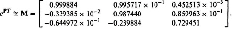
In this example, b = 4. When K = 9, the upper bound of |r_ij| from Eq. (2.338) is 0.587945 × 10⁻⁷. Therefore, 10^b|r_ij| = 0.587945 × 10⁻³ < |m_ij|, (i,j = 1, 2,...), where m_ij are the elements of M given in the example. This illustrative example indicates the simplicity and accuracy of the procedure for obtaining the state transition matrix utilizing its series definition.