6.12.  RELATIONSHIP BETWEEN CLOSED-LOOP FREQUENCY RESPONSE AND THE TIME-DOMAIN RESPONSE

Section 6.10 has illustrated how the closed-loop frequency-domain response may be obtained from the open-loop transfer function. The next logical question to ask is how to determine the relationship between M_p and the peak overshoot one obtains in the time domain. In Chapter 4, we defined the time at which the peak overshoot occurs as t_p in terms of ζ and ω_n [see Eq. (4.29)]. For example, does an M_p of 1.3 mean a 30% transient overshoot in the time domain?

Table 6.20. MATLAB Program to Obtain the Nichols Chart for the System whose Open-Loop Transfer Function is shown in Eq. (6.121)

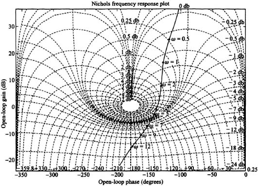
Figure 6.52   Nichols chart with superimposed.

This problem has been analyzed for the general, unity-feedback system of Figure 6.45 [22]. After determining the Fourier transform of the input, R(ω), and that of the output, C(ω), the value of C(ω) was then related to the transient response in the time domain. The resulting approximate general relationship between M_p and the peak overshoot of the transient in the time domain has been shown [22] to be given by

Therefore, the overshoot in the time domain is, in general, related to M_p by some factor equal to or less than 18%. This approximation is extremely important, because it permits the control-system engineer to correlate peak overshoots in the frequency and time domains.

For second-order systems, exact relationships can be obtained for M_p and ω_p in terms of the damping factor ζ. In order to derive this expression, let us reconsider the closed-loop transfer function of a second-order system in the following form:

Therefore, the magnitude of the closed-loop response is given by

In order to find the maximum value M_p of M, and the frequency at which it occurs, ω_p, Eq. (6.124) is differentiated with respect to frequency and set equal to zero. The frequency ω_p at which M_p occurs is found to be given by

If this value of ω_p is substituted into Eq. (6.124), the value of M_p is found to be given by

A plot of M_p versus ζ is illustrated in Figure 6.53. Observe from this figure that M_p increases very rapidly for ζ < 0.4. The resulting transient oscillatory response is excessively large in this region, and is undesirable from practical considerations. Therefore, systems having a ζ < 0.4 are not normally desired. In electro-mechaical systems, values of M_p in the range of

1 < M_p < 1.4

are usually specified, which requires ζ > 0.4 if the system is a pure second-order system. In industrial process control, values of M_p up to 2.0 are often used.

Let us carry the analysis of the second-order system one step further by correlating its frequency- and time-domain response. In Section 4.2, we found that the peak value of c(t) for the step response of a second-order system is given by [see Eq. (4.32)]

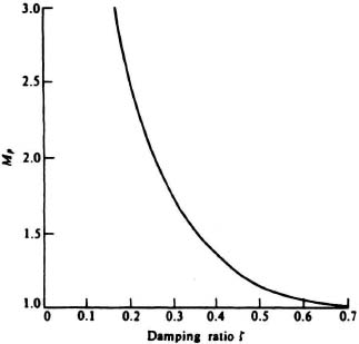
Figure 6.53   M_p versus the damping ratio.

To check the correspondence between M_p [from Eq. (6.126)] and c(t)_max [from Eq. (6.127)], consider the case where ζ = 0.4. Substituting into Eqs. (6.126) and (6.127),

and they are within 18% of each other as stated in Eq. (6.122). Actually, the difference is only 8.76%. As the damping factor ζ increases, the correspondence gets better. For example, if ζ = 0.6, then M_p = 1.04 and c(t)_max = 1.09; a difference of only 4.8%. In general, when ζ > 0.4, there is a close correspondence between M_p and c(t)_max. For values of ζ < 0.4, the correspondence between M_p and c(t)_max is only qualitative. For example, for the second-order system and at ζ = 0.1, we find that M_p = 5.03 and c(t)_max = 1.73. However, because practical second-order systems usually do not use a ζ < 0.4, the 18% relationship given in Eq. (6.122) is quite accurate for systems of interest.