2.19.  SIMULATION DIAGRAMS

From the development of signal-flow graphs, Mason’s theorem, and operational amplifiers, we can now develop simulation diagrams. The simulation diagram can be either a block diagram or a signal-flow graph which is constructed to have a specified transfer function or to model a set of specified differential equations. The resulting simulation diagram is very useful because it can be used to construct either a digital computer or analog computer simulation of the control system.

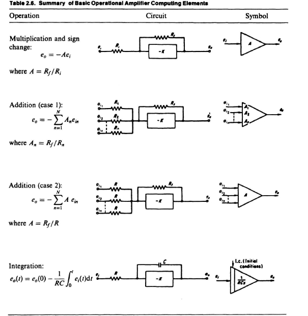
From the previous section on operational amplifiers, the basic element of the simulation diagram is an integrator (see Eq. (2.143) and Table 2.6). In using the integrator in a simulation diagram, therefore, it is important to recognize that if the output of the integrator is x(t), then the input to the integrator is dx(t)/dt. Similarly, if two integrators are connected in cascade and the output of the last integrator is x(t), then the input to the last integrator is dx(t)/dt, and the input to the first integrator is d²x(t)/dt². We can use integrators, amplifiers, and summers, which were all described in Section 2.18 on operational amplifiers and summarized in Table 2.6, to represent a given differential equation by a simulation diagram.

In addition to representing a differential equation by a simulation diagram, we can reverse this procedure and start with a given transfer function to construct the simulation diagram. A simulation diagram constructed from a differential equation representing the system is usually unique. If the simulation diagram is constructed from the transfer function, however, the simulation diagram is not unique. This is illustrated next.

Let us consider representing the closed-loop transfer function

by a simulation diagram. It can be accomplished by Figures 2.23 or 2.24. Both are correct. Figure 2.23 is denoted as the observer-canonical form, and Figure 2.24 is denoted as the control-canonical form. We use the term observer-canonical form to denote the configuration in Figure 2.23 because all the feedback loops come from the output or the “observed” signal. We use the term control-canonical form to denote the configuration in Figure 2.23 because all the feedback loops come from the output or the “observed” signal. We use the term control-canonical form to denote the configuration in Figure 2.24 because all the feedback loops return to the input or the “control” variable. Applying Mason’s theorem to these two simulation diagrams, we find that they both have the same transfer function. For example, from the observer-canonical form of Figure 2.23, we find that

Figure 2.23   Observer-canonical form representation of Eq. (2.149).

Figure 2.24   Control-canonical form representation of Eq. (2.149).

For the control-canonical form of Figure 2.24, we find that

Therefore, we conclude that simulation diagrams constructed from transfer functions are not unique, and can have different forms.