2.22.  STATE-VARIABLE DIAGRAM

The state-variable diagram provides a physical picture that is useful in understanding the state-variable concept. In addition, the differential equations relating the state variables are easily obtained by inspection of the diagram. A state-variable diagram consists of integrators, summing devices, and amplifiers. Outputs from the integrators denote the state variables. It should be noted that the state-variable diagram is the same as an analog computer simulation diagram [15].

Example 1. As an example of determining the state-variable diagram, consider a system whose transfer function is given by

Dividing numerator and denominator by s³, to obtain the result in terms of integrators:

Defining the error node of the control system to be E(s),

Eq. (2.223) may be rewritten as follows:

From Eq. (2.225) and the relation

the state-variable diagram can easily be obtained as indicated in Figure 2.30*. The state variables are indicated in the diagrams as x₁(t), x₂(t), and x₃(t). Also, the differential equations relating the state variables are easily obtained from Figure 2.30 by inspection. From the state-variable diagram, the differential equations relating the state variables are as follows:

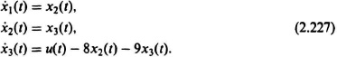
Therefore, the entire system can be described in phase-variable canonical form by

Figure 2.30   State-variable diagram for system where P(s) = (s² + 4s + 1)/(s³ + 9s² + 8s).

where

The output c(t) can be obtained by a linear combination of the three state variables as follows:

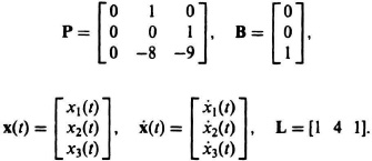
Example 2. As a second example for determining the state-variable diagram, consider a system whose transfer function is given by

Dividing through by s⁴ we obtain

Defining

Eq. may be rewritten us

From Eq. (2.233) and the relation

the state-variable diagram for this system can easily be obtained (see Figure 2.31). The state variables are referred to as x₁(t), x₂(t), x₃(t), and x₄(t). They are defined as

The differential equations relating the state variables are as follows:

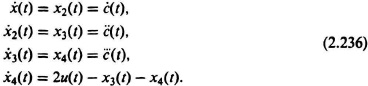
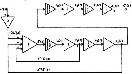
Figure 2.31   State-variable diagram for system where P(s) = [2/s²(s² + s + 1)].

The corresponding phase-variable canonical form is given by

where

From this discussion it can be seen that it is possible to apply the signal-flow graph technique to state-variable analysis. Mason’s theorem can be applied to the signal-flow graph which is obtained directly by inspection of the state-variable diagram. The signal-flow graph also provides a physical interpretation of the state-variable concept since its nodes actually represent the different states of the system.

For example, the signal-flow graphs corresponding to the state-variable diagrams of Figures 2.30 and 2.31 are given in Figures 2.32 and 2.33, respectively. The physical meaning of system state is quite clear from these diagrams.