8.3.  CONTROLLER DESIGN USING POLE PLACEMENT AND LINEAR-STATE-VARIABLE FEEDBACK TECHNIQUES

The preceding section has indicated several important relationships between open-loop and closed-loop transfer functions. This is very important in the design of control systems for the case where the closed-loop transfer function is specified and it is desired to determine the open-loop transfer function. A typical problem might specify the desired velocity constant; then use is made of Eq. (5.35) in Section 5.4 which gave the velocity constant in terms of the closed-loop poles and zeros. The problem is to determine the resulting linear-state-variable feedback system.

Let us illustrate the procedure by considering the following problem. It is desired that the closed-loop characteristics of a unity-feedback control system be given by the following parameters:

ω_n = 50 rad/sec,      K_v = 35/sec,      ζ = 0.707

What form of closed-loop transfer function will satisfy these requirements? Let us first try a simple quadratic control system having a pair of complex-conjugate poles. From Eq. (5.37), such a system has a velocity constant given by

Therefore, a simple quadratic control system having a pair of complex-conjugate poles will satisfy these specifications. From Eq. (4.18),

For a damping ratio of 0.707, α = 45° and the relations among the complex-conjugate poles, ω_n and ζ are illustrated in Figure 8.6. Therefore, the closed-loop control system is given by

Figure 8.6  Closed-loop poles.

By substituting ζ = 0.707 and ω_n = 50 into Eq. (8.27), we obtain the following desired closed-loop transfer function:

Let us assume that the open-loop process that is being controlled is illustrated in Figure 8.7. The corresponding state-variable representation is readily found to be

where

The resulting linear-state-variable feedback representation is illustrated in Figure 8.8. This feedback represenation can be simplified by the configuration illustrated in Figure 8.9. The resulting closed-loop transfer function is given by

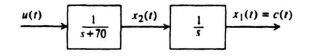
Figure 8.7  Open-loop process to be controlled.

Figure 8.8  State-variable feedback representation of system.

which can be reduced to the following expression:

The values of K₁h₁ and h₂ can be found from Eqs. (8.28) and (8.32). The following set of simultaneous equations result:

We have three equations and three unknowns. Solving, we find that h₁ = 1, K = 2500, and h₂ = 2.8 × 10⁻⁴. The final step is to draw the root locus and examine the relative stability, and the sensitivity as a function of slight gain variations. For this simple system, the final step is not necessary.

Although this simple example has been solved using block diagrams and transfer functions, it could also have been solved using the matrix-algebra approach. To illustrate this, let us pick up this problem from Eq. (8.28) which is the desirable closed-loop transfer function. We want to determine the closed-loop transfer function for the linear-state-variable-feedback control system using Eq. (8.18) and knowledge of the P and B matrices from Eq. (8.29), and the matrix L from Eq. (8.30) as follows:

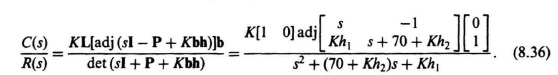
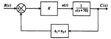
Figure 8.9  Equivalent configuration of Figure 8.8.

Simplifying Eq. (8.36), we obtain the following:

Simplifying Eq. (8.37) results in the following expression for the closed-loop transfer function of the system:

Equation (8.38) is identical to the closed-loop transfer function we obtained in Eq. (8.32) which was obtained from the block diagram shown in Figure 8.8. Therefore, we repeat the process of setting like terms equal to each other from Eq. (8.38) and Eq. (8.28). The resulting three simultaneous equations of (8.33) through (8.35) will be identical, and the resulting parameters of K = 1, h₁ = 1, and h₂ = 2.8 × 10⁻⁴ will be the same as found before.

With this fundamental example as a basis, the general pole placement design procedure can be formulated as follows:

1. Determine the desired closed-loop transfer function based on the discussion of Section 5.4.
2. Determine the representation of the process to be controlled.
3. Represent the closed-loop system in terms of an equivalent linear-state-variable-feedback configuration.
4. Determine the closed-loop transfer function C(s)/R(s) from the equivalent model in terms of K and h.
5. Equate the C(s)/R(s) expressions from Steps 1 and 4 and determine K and h.^*
6. Plot the resulting root locus of KG(s)H(s) and evaluate the relative stability and sensitivity as a function of gain variations.

Let us apply this pole placement procedure next to the following more complex example. The problem concerns the control of a process in a unity-feedback closed-loop system whose transfer function is given by

It is assumed that the transient response of the system is governed by a pair of dominant complex-conjugate poles, and that the following parameters are desired:

K_v = 0.93,
    ζ = 0.707,
       ω_n = 1 rad/sec.

What should the closed-loop transfer function be? From Eq. (5.37), a pair of complex-conjugate poles in the denominator would only have a velocity constant given by

Therefore, a simple pair of complex-conjugate poles is inadequate to meet the velocity constant requirement of 0.93. By examining Eq. (5.35), we conclude that a zero Z must be added to the closed-loop transfer function. How many poles should the closed-loop system have? Because

where

N_Pc = number of closed-loop poles = ?
  N_zc = number of closed-loop zeros = 1,
N_P0 = number of open-loop poles = 3, 
N_z0 = number of open-loop zeros = 0  

therefore

and

Since the resulting unity-feedback, closed-loop transfer function has to have one zero and four poles, it has the following general form:

The value of the zero Z can be found from Eq. (5.35) as follows:

Due to external overall system factors in which this feedback system is to operate, it is assumed that the poles at P₃ and P₄ are specified to occur at 9 and 16, respectively.
Therefore,

so that Z = 2, and the desired closed-loop transfer function is given by

or

Because the zeros of G(s) must be the same as that of C(s)/R(s), we must also add the factor (s + 2) to the numerator of G(s). Then, to satisfy Eq. (8.41), we must add a pole factor (s + α) to the denominator of G(s). The resulting compensating network to be added to G(s) is given by

where α is a pole of the open-loop transfer function which is to be determined. The resulting linear-state-variable feedback system is illustrated in Figure 8.10. The problem remaining is to select the values of K, α, and h.

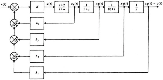
Figure 8.10  State-variable feedback representation of system.

An equivalent block diagram of this system is illustrated in Figure 8.11. The resulting closed-loop transfer function from this equivalent model is given by

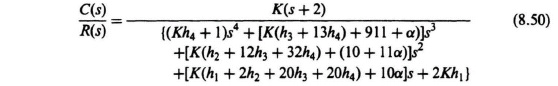
Equating the two forms of C(s)/R(s) given by Eqs. (8.48) and (8.50), the following set of equations is obtained:

                                                 K = 72,
                                     Kh₄ + 1 = 1,
                 K(h₃ + 13h₄) + (11 + α) = 26.4,
  K(h₂ + 12h₃ + 32h₄) + (10 + 11α) = 180.4,
  K(h₁ + 2h₂ + 20h₃ + 20h₄) + 10α = 229,
                                               2Kh₁ = 144.

Notice that we have six simultaneous equations with six unknowns (K, h₁, h₂, h₃, h₄, and α). Solving these equations, we obtain the following expressions:

From Eq. (8.49), the resulting compensation network, G_c(s), is given by

which is a phase-lead network.

It is important to emphasize that α could have turned out to be negative for a different set of specifications This would be undesirable, because it would result in a zero in the right-half plane; this system would be unstable. In other cases, the system might be conditionally stable.

Our results of this pole placement example can be evaluated most conveniently on a root-locus plot. To obtain the root locus of the compensated system, the open-loop transfer function will be obtained. For the values of the parameters found in Eq. (8.51), H(s) results in the following:

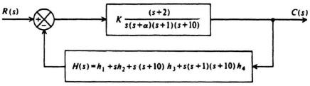
Figure 8.11  Equivalent block diagram for system illustrated in Figure 8.10.

Combining Eqs. (8.39), (8.52), and (8.53) we obtain the following transfer function for the open-loop system:

The resulting root locus is plotted in Figure 8.12. Observe that the resulting root locus is stable for all values of K from zero to infinity. The locations of the dominant complex-conjugate roots for K = 72 are indicated.

It is important to emphasize again that the discussion of linear-state-variable feedback in this and the preceding section has assumed that all of the state variables are accessible. This is not always the case. This is analyzed further in Sections 8.6 and 8.7.