8.4.  CONTROLLABILITY

The presentation of linear-state-variable feedback in Sections 8.2 and 8.3 assumed that all of the states are observable and measurable, and available to accept control signals (controllable). The concepts of controllability [2–4], and observability also play a very important role in optimal control theory (presented in the accompanying volume). Before designing a control system, we must determine whether it is controllable and its states are observable, since the conditions on controllability and observability often govern the existence of a solution to an optimal control system. Kalman [2,3] first introduced the concepts of controllability and observability in 1960. These concepts are basic in modern optimal control theory. This section develops mathematical tests to determine controllability, and the following section presents mathematical tests for determining observability.

Figure 8.12  Root locus for the system of Figure 8.11 with the parameters of Eq. (8.51).

In order to introduce the concept of controllability, let us consider the simple open-loop system illustrated in Figure 8.13. A system is completely controllable if there exists a control which transfers every initial state at t = t₀ to any final state at t = T for all t₀ and T. Qualitatively, this means that the system G(s) is controllable if every state variable of G can be affected by the input signal u(t). However, if one (or several) of the state variables is (or are) not affected by u(t), then this (or these) state variable(s) cannot be controlled in a finite amount of time by u(t) and the system is not completely controllable.

A.  Controllability by Inspection

As an example of a system which is not completely controllable, let us consider the signal-flow diagram illustrated in Figure 8.14. This system contains four states, only two of which are affected by u(t). This input only affects the states x₁(t) and x₂(t). It has no effect on x₃(t) and x₄(t). Therefore, x₃(t) and x₄(t) are uncontrollable. This means that it is impossible for u(t) to change x₃(t) from initial state x₃(0) to final state x₃(T) in a finite time interval T and the system is not completely controllable.

B.  The Controllability Matrix

Let us now consider this problem more precisely and establish a mathematical criterion for determining whether a system is controllable. We limit our discussion to linear constant systems. Assume that the system is described by

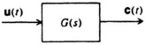
Figure 8.13  Open-loop system containing several inputs and outputs.

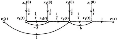
Figure 8.14  Signal-flow graph of a system that is not completely controllable.

The solution of Eq. (8.55) can be expressed as Eq. (2.265):

Let us assume that the desired final state of our system at t = t_f is zero:

Using Eqs. (2.259) and (2.261), we can write Eq. (8.57) as

The state-transition matrix can be expressed from Eq. (2.322) as

Here, x is an m × 1 vector, P is an m × m matrix, u is an r × 1 vector, B is an m × r matrix, and α_n(t) is a scalar function of t. (This form results from application of the Cayley–Hamilton theorem). Substituting Eq (8.60) into Eq (8.59), we obtain the following expression for x(t₀):

Because the matrices P and B are not functions of τ, we can rewrite Eq (8.61) as

Equation (8.62) can be rewritten as

where

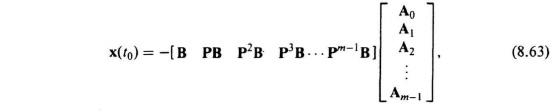
If we define

where D, the controllability matrix, is an m × mr matrix and A is an mr × 1 vector, then Eq (8.63) becomes

For a given initial state x(t₀), the input u can be found to drive the state to x(t_f) = 0 for a finite time interval t_f − t₀ if Eq (8.67) has a solution. A unique solution occurs only if there is a set of m linearly independent column vectors in the matrix D. If u is a scalar, then D is an m × m square matrix, and Eq (8.67) represents a set of m linearly independent equations which have a solution if D is nonsingular or the determinant of D is not zero. The controllability criterion thus states that the system of Eqs. (8.55) and (8.56) is completely controllable if D [see Eq (8.65)] contains m linearly independent column vectors or, if u is a scalar, D is nonsingular.

In order to illustrate this mathematical controllability concept, consider a second-order system where

and

Then, from Eq (8.65),

The resulting matrix D is singular (its determinant is zero) and the system is therefore not completely controllable.

As a second example, consider a second-order system where

and

Then, from Eq. Eq. (8.65)

The resulting matrix D is nonsingular and the system, therefore, is completely controllable.