
8.14. ILLUSTRATIVE PROBLEMS AND SOLUTIONS
This section provides a set of illustrative problems and their solutions to supplement the material presented in Chapter 8.
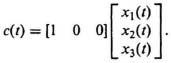
I8.1. The state and output equations of a second-order control system are given by the following:
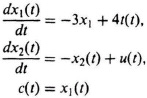
where x1(t) and x2(t) represent the system states, c(t) is the system’s output, and u(t) represents its input.
(a) Determine whether the system is controllable.
(b) Determine whether the system is observable.
SOLUTION: (a) From Eq. (8.65) controllability can be determined for this second-order system from:
D = [B PB].
The phase variable canonical form of the state and output equations can be written as:

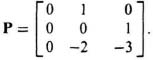
Therefore the companion matrix, P is given by
![]()
and the input vector, B, is given by

and the output matrix is given by:
L = [1 0]
Therefore, the matrix D is given by:
![]()
and the system is controllable.
(b) Observability can be determined for this second-order control system from Eq. (8.75) where
U = [LT PTLT]
Therefore, the matrix U is given by:
![]()
So, the system is unobservable because U is singular.
I8.2. Synthesize a system using linear-state-variable feedback that has a closed-loop transfer function given by
![]()
Assume that the proces to be controlled has a transfer function given by
![]()
In your solution, show the following:
(a) Synthesis of the linear-state-variable-feedback system.
(b) Identification of any compensation network needed to satisfy the synthesis. What kind of network is it?
(c) Check of the stability of the resulting system synthesized using the root-locus method.
.jpg)
Figure I8.2(i)

This equation can be reduced to the following:
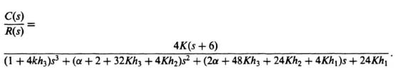
Comparing the coefficients of this equation for the synthesized linear-state-variable-feedback system and that of the desired closed-loop transfer function given by
![]()
we obtain the following five simultaneous equations to be solved:
10 = 4k,
1 + 4kh3 = 1,
α + 2 + 32Kh3 + 4KH2 = 4,
2α + 48Kh3 + 24Kh2 + 4Kh1 = 10,
24Kh1 = 20.
Therefore, we obtain the following results:
K = 2.5; h1 = 0.33; h2 = 0.0675; h3 = 0; α = 1.325.
(b) The compensation network is given by
![]()
which is a phase-lag network.
(c) The root locus is drawn from the following transfer function:
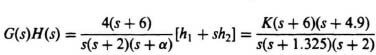
The following root-locus diagram shows that this control system is stable for 0 < K < ∞:
.jpg)
Figure I8.2(ii)
I8.3. Design a third-order controller whose three roots are located at the following locations in the s-plane: −1; −1; −12. The transfer function of the system to be controlled is given by
![]()
Determine the controller gain matrix, K.
SOLUTION: The desired location of the controller roots are located at:
We need to determine the companion matrix, P, and the input gain vector, b, so that we can solve for the controller gain matrix, K from Eq. (8.167). The states of this third-order control system are defined as follows:
Let x1; = c(t); x2 = ![]() (t); x3 =
(t); x3 = ![]() (t). Therefore, the state equations are given by:
(t). Therefore, the state equations are given by:
![]() 1(t) = x2(t),
1(t) = x2(t),![]() 2(t) = x3(t),
2(t) = x3(t),
![]() 3(t) = –8x1(t) – 2x2(t) – 3x3(t) + u(t).
3(t) = –8x1(t) – 2x2(t) – 3x3(t) + u(t).
The state equations in their vector and matrix format are given by:
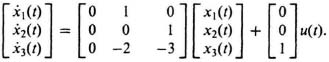
Therefore, the companion matrix, P, is given by:
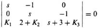
The controller gain K can be determined from Eq. (8.167) as follows:
|sI − P + bK| = 0
Substituting into Eq. (8.167), we obtain the following:

This can be simpified to
which can be reduced to the following:
Setting coefficients of Eqs. (I8.3-1) and (I8.3-2) equal to each other, we obtain the following:
14 = 3 + K3,
25 = 2 + K2,
12 = K1.
Therefore, we solve these three equations and find that:
K1 = 12,
K2 = 23,
K3 = 11.
Therefore, the controller gain matrix, K, is given by:
K = [12 23 11].
I8.4. Design a third-order estimator whose three roots are located at the following locations in the s-plane: −3.5; −3.5; −15. The transfer function of the process is given by
![]()
Determine the estimator gain vector M.
SOLUTION: The desired location of the estimator roots is at:
We need to determine the companion matrix, P, the input gain vector, b, and the output matrix, L, so that we can determine the estimator gain factors in the M matrix from Eq. (8.131). The states of this third-order control system are defined as follows:
Let x1(t) = c(t); x2(t) = ![]() (t); x3(t) =
(t); x3(t) = ![]() (t). Therefore, the state equations are given by:
(t). Therefore, the state equations are given by:
![]() 1(t) = x2(t),
1(t) = x2(t),![]() 2(t) = x3(t),
2(t) = x3(t),
![]() 3(t) = –12x2(t) – 7x3(t) + r(t).
3(t) = –12x2(t) – 7x3(t) + r(t).
The state equations in their vector and matrix form are given by:
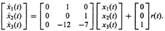
Therefore, the companion matrix, P and the input vector, b, are
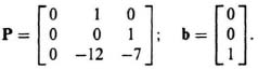
The output equation is given by:
Therefore, the output matrix is given by
L = [1 0 0].
The M matrix can be determined from Eq. (8.131) as follows:
|sI − (P − ML)| = 0
Substituting into Eq. (8.131), we obtain the following:
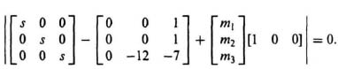
This can be simplified to
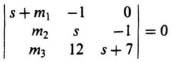
which can be reduced to the following:
Setting like coefficients of Eqs. (I8.4-1) and (I8.4-2), equal to each other, we obtain the following:
22 = 7 + m1,
117.25 = 12 + 7m1 + m2,
183.75 = 12m1 + 7m2 + m3.
Therefore, we solve these equations and find that:
m1 = 15,
m2 = 0.25,
m3 = 2.
Therefore, the M vector is given by:

I8.5. Repeat the problem solved in Section 8.6 using Ackermann’s Formula for a process transfer function given by
![]()
and the control system’s signal flow graph is given by:
.jpg)
Figure I8.5(i)
(a) Determine the state equations for the process.
(b) Determine the controllability matrix for this original system.
(c) Transform the original system to the phase variable form, and determine the state and output equations.
(d) Determine the controllability matrix for the phase variable form.
(e) Determine the transformation matrix A.
(f) Design a contoller assuming that the dominant pair of complex-conjugage roots has a damping ratio of 0.707, and it results in a settling time of 4 sec. Select the third pole at the location of the zero of the process to be controlled. What is the resulting characteristic equation of the desired closed-loop control system?
(g) Determine the state and ouput equations for the phase-variable form with linear-state-variable-feedback.
(h) What is the resulting characteristic equation for the set of equations found in part (g)?
(i) Determine the linear-state-variable-feedback constants for the control system in phase-variable form.
(j) Transform the linear-state-variable-feedback constants back to the original system using the transformation matrix A.
(k) Draw the resulting closed-loop control system with linear-state-variable-feedback.
SOLUTION: (a)
(b) 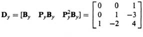
The value of the determinant of Dy is –1, it’s nonsingular, and the original control system is controllable as expected from inspection of the signal-flow graph.
(c) From the given signal-flow graph:

This transfer function can be reduced to the following:
![]()
Defining x1(t) = c(t), x2(t) = ![]() (t), and x3(t) =
(t), and x3(t) = ![]() (t), we obtain
(t), we obtain
![]() 1(t) = x2(t)
1(t) = x2(t) ![]() 2(t) = x3(t)
2(t) = x3(t)
![]() 3(t) = 14x1(t) – 23x2(t) – 10x3(t) + 3u(t) +
3(t) = 14x1(t) – 23x2(t) – 10x3(t) + 3u(t) + ![]() (t)
(t)
Therefore, the state and output equations in matrix vector form of the phase variable control system are given by:

(d) The resulting controllability matrix for the phase variable form can be obtained from
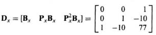
Note that the determinant of Dx is −1 indicating that the determinant is nonsingular, and the phase variable form is also controllable, as expected.
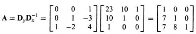
(e) The transformation matrix, defined in Eq. 8.85 is
(f) A second-order control system having a damping ratio of 0.707 with a settling time of 4 seconds results in a ωn = 1.414 (see Eq. 5.41). Therefore, the following second-order control system can meet the design specifications:
![]()
With third pole selected at s = 3, which also cancels the zero at s = −3, the characteristic equation of the desired closed-loop system is given by:
(s2 + 2s + 2)(s + 3) = s3 + 5s2 + 8s + 6 = 0
(g) The state and output equations for the phase-variable form with linear-state-variable-feedback can be obtained from Eqs. 8.8 and 8.10 as follows:

The state equation reduces to the following:
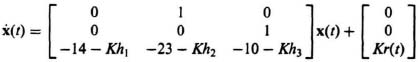
(h) The resulting characteristic equation can be obtained from Eqs. 8.10 and 8.19:
det(sI − Ph) = (sI − P + Kbh) = 0
Therefore,

The resulting characteristic equation is given by:
s3 + (10 + Kh3)s2 + (23 + Kh2)s + (14 + Kh1) = 0
(i) Comparing this characteristic equation (see part h) with the characteristic equation of the desired closed-loop system (see part f), results in the following:
10 + Kh3 = 5; Kh3 = −5
23 + Kh2 = 8; Kh2 = −15
14 + Kh1 = 6; Kh1 = −8
Therefore,
Khx = [−8 −15 −5]
(j) We will now transform Khx back to the original system using Eq. 8.94 as follows:
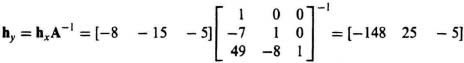
(k) The resulting closed-loop control system with linear-state-variable-feedback is the following:
.jpg)
Figure I8.5(ii) Resulting closed-loop control system with linear-state-variable-feedback designed using Ackermann’s formula.
I8.6. Design a combined compensator of a regulator containing a controller and estimator for the system illustrated in Figure I8.6(i).
.jpg)
Figure I8.6(i)
Assume that the transfer function of the process is given by
![]()
Assume that the design specification of the controller is that it is critically damped with ωn = 3 rad/sec, and that the estimator is also critically damped with ωn = 30 rad/sec.
(a) Find the controller’s gain coefficients’ matrix.
(b) Find the estimator’s coefficients’ vector.
(c) Determine the transfer function of the compensator for the combined controller and estimator, U(s)/C(s).
(d) Sketch the root locus of the compensated system. From your sketch, is the system unstable, stable, or conditionally stable?
SOLUTION: (a) The desired location of the controller roots is at:
We need to determine the companion matrix, P, and the input gain vector, b, so that we can solve for the controller gain matrix, K, from Eq. (8.167). The states of this second-order control system are defined as follows:
Let x1(t) = c(t); x2(t) = ![]() (t). Therefore, the state equations are given by:
(t). Therefore, the state equations are given by:
![]() 1(t) = x2(t)
1(t) = x2(t) ![]() 2(t) = −4x1(t) − 4x2(t) + 4u(t).
2(t) = −4x1(t) − 4x2(t) + 4u(t).
The state and output equations in their vector and matrix format are given by:
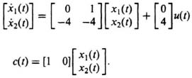
Therefore, the companion matrix, P, the input vector, b, and the output matrix, L are given by:
![]()
The controller gain K can be determined from Eq. (8.167) as follows:
|sI − P + bK| = 0.
Substituting into Eq. (8.167), we obtain the following:

This equation can be simplified to
![]()
which can be reduced to the following:
Setting like coefficients of Eqs. (I8.6-1) and (I8.6-2) equal to each other, we obtain the following:
6 = 4(1 + K2),
9 = 4(1 + K1).
Therefore, we solve these two equations and find that:
K1 = 1.25
K2 = 0.5
Therefore, the controller gain matrix, K, is given by:
K = [1.25 0.5]
(b) The desired location of the estimator roots is at:
The M matrix can be determined from Eq. (8.131) as follows:
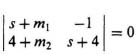
|sI − (P − ML)| = 0
Substituting into Eq. (8.131), we obtain the following:
![]()
This can be simplified to
which can be reduced to the following:
Setting like coefficients of Eqs. (I8.6-3) and (I8.6-4) equal to each other, we obtain the following:
60 = m1 + 4; m1 = 56
900 = 4m1 + 4 + 4m2; m2 = 672.
Therefore, the M vector is given by:
![]()
(c) The transfer function of the compensator, U(s)/C(s) can be determined from Eq. (8.162):
![]()
Substituting values for K, P, B, and L found in part (a), and M found in part (b), we obtain the following:
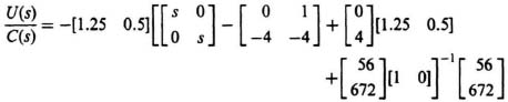
which reduces to
![]()
Further reduction reduces this equation to the following:
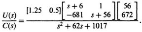
This equation reduces the following expression for the transfer function of the compensator for the combined controller and estimator, U(s)/C(s):
![]()
This is a phase-lead network having the zero at s = −2.48.
(d) The root locus for the compensated system is plotted from the following expression:
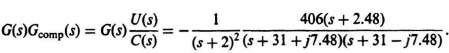
The root locus shown in Figure I8.6(ii) shows that this is a conditionally stable system that is stable for < K < 61, 102. Observe that the root locus goes through the roots chosen for the controller roots (s = −3, −3) and estimator roots (s = −30, −30).
.jpg)
Figure I8.6(ii)
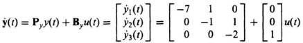
I8.7. The system of Problem I8.6 is modified to respond to a reference input, r(t), as shown in the following block diagram:
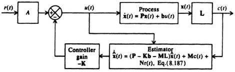
Figure I8.7
Assume that the process, combined compensator containing a controller and an estimator, and the specifications for the controller and estimator are exactly the same as in Problem I8.6. Assuming that A = 4, determine the requirement on M so that the state-estimation error is independent of the reference input, r(t).
SOLUTION: We can determine the requirement on N so that the state-estimation error is independent of the reference input, r(t), from Eq. (8.193):
bA = N.
From Problem I8.6, we know that the input vector, b, is given by
![]()
Substituting b and A = 4 into Eq. (8.193), we obtain the following:
![]()
Therefore, N is given by
![]()
I8.8. We wish to design a robust control system containing a two-degrees-of-freedom series controller Gcl(s) and a forward-loop-controller Gc2(s) which is illustrated as follows:
.jpg)
Figure I8.8(i)
The transfer function KG0(s) is
The gain of this transfer function can vary significantly, and the value of 150 is only the nominal amount. During its operation, the gain has been known to go as low as 75 and as high as 300. The objective of the control-system engineer is to design the robust control system shown so that the effect of this wide gain variation is minimized on the control system’s transient response.
(a) Determine the control system’s transient response to a unit step input for K = 75, 150, and 300, assuming that Gc1(s) = Gc2(s) = 1.
(b) Draw the root locus for the conditions defined in part (a).
(c) From the root locus drawn in part (b), determine the location of the roots for the closed loop system for gains of 75, 150, and 300, and the damping and overshoot, for the dominant set of complex-conjugate roots, for the three sets of gains being considered.
(d) Design the robust controller Gc2(s).
(e) Determine the transfer function KGc2(s)G0(s).
(f) Plot the root locus for the transfer function determined in part (e), and determine the damping, overshoot, and the roots of the characteristic equations for gains of 75, 150, and 300.
(g) Determine the design of the forward-loop controller Gc1(s) in this two-degrees-of-freedom control system.
(h) With Gc1(s), as determined in part (g) added to this control system, determine the transient response of this control system to a unit step input for K = 75, 150, and 300.
(i) What conclusions can you reach from the resulting transient responses found in parts (a) and (h)?
SOLUTION: (a) Figure I8.8(ii) illustrates the unit step responses for this control system for K = 75, 150, and 300 which was obtained using MATLAB. Observe from this figure that the peak overshoot varies from 27.3% for K = 75, to 69.3% for K = 150, and 76.3% for K = 300.
(b) The root locus obtained from MATLAB is shown in Figure I8.8(iii).
(c) Table I8.8(i) lists the damping, overshoot, and the characteristic equation roots for the dominant set of complex-conjugate roots of this control system.
Observe from this table the considerable variation in the damping ratio and the maximum percent overshoot (based on the dominant complex-conjugate roots) for the three cases being analyzed.
(d) The robust controller has the following pair of complex-conjugate zeros to cancel the poles of the system where K = 150:
.jpg)
Figure I8.8(ii) Unit step response of KG(s) = K(s + 12)/(s + 2)(s + 8)(s + 25).
.jpg)
Figure I8.8(iii) Root-locus plot for system shown in Figure I8.8(i) for KG0(s) as defined in Eq. (I8.8-1) and Gc1(s) = Gc2(s) = 1.
.jpg)
.jpg)
Figure I8.8(iv) Root-locus plot for system shown in Figure I8.8(i) with KGc2(s)G0(s) given by Eq. (I8.8-3).
.jpg)
Figure I8.8(v) Unit step response of KG(s) = K(s + 12)/s(s + 2)(s + 8)(s + 25) with robust control.
.jpg)
(e)
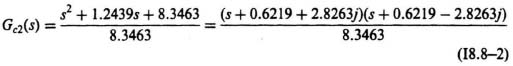
(f) The root locus, which was obtained using MATLAB, is illustrated in Figure I8.8(iv). From this root locus, the damping ratio, maximum percent overshoot, and roots of the characteristic equation are shown in Table I8.8(ii):
(g) The design of the forward-loop controller Gc1(s) is the reciprocal of the robust controller Gc2(s):
(h) The resulting transient response of this control system to a unit step input for K = 75, 150, and 300 is illustrated in Figure I8.8(v).
(i) The resulting transient response illustrated in Figure I8.8(v) shows that the maximum percent overshoots with the robust control design have been greatly reduced from those illustrated in Figure I8.8(ii). The new robust control-system design truly exhibits admirable robust control features. Table I8.8(iii) compares the transient response with and without robust control:
| K | Maximum percent overshoot without robust control | Maximum percent overshoot with robust control |
| 300 | 76.3% | 40.2% |
| 150 | 69.3% | 31.7% |
| 75 | 27.3% | 19.9% |
In addition to the reduction in the maximum percent overshoots, observe that the range of the maximum percent overshoots is reduced from 76.3%/27.3% = 2.79 without robust control to 40.2/19.9% = 2.02. That is a very significant reduction which robust control makes possible. Therefore, the robust system is much less sensitive to variations in K. In addition, the robustness with respect to variations in K will also provide disturbance suppression to D(s).
I8.9. The optimal sensitivity function for the control system illustrated in Figure I8.9(i) is to be determined in the H∞ sense.

Figure I8.9(i)
The transfer function of the process G(s) is given by
![]()
The weighting function W(s) is given by
![]()
(a) Determine the value of Bp(s).
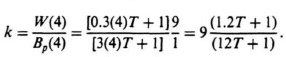
(b) Determine the value of the constant k.
(c) Determine the value of the optimal sensitivity function S(s).
(d) Determine the absolute value of the optimal sensitivity function and plot the results for T = 0.2, 2, and 20 sec.
(e) What conclusions can you reach from these curves?
SOLUTION: (a) From Eq. (8.252), the right-half pole of G(s) at s = 5 results in
![]()
(b) Because G(s) has only one zero in the right half-plane of the s-plane, then B′(s) = 1. Therefore, from Eq. (8.254), we can find k as follows:
(c) Substituting into Eq. (8.256) for k, B′(s), Bp(s), and W(s), we obtain the following:
(d) The absolute value of the optimal sensitivity function can be obtained from Eq. (8.257) as follows:
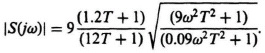
The absolute value of the sensitivity function is plotted in Figure I8.9(ii) for the following values of T: 0.2, 2, and 20.
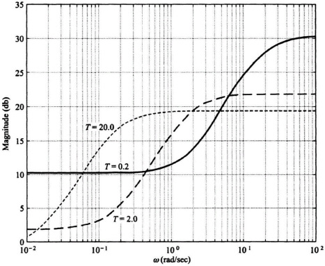
Figure I8.9(ii) Optimal sensitivity frequency characteristic as a function of T.
(e) It is concluded from these curves that the sensitivity is smaller (better) at low frequencies if the bandwidth is not too high (or T is not too small).