2.2  REVIEW OF COMPLEX VARIABLES, COMPLEX FUNCTIONS, AND THE s PLANE

The design of control systems depends greatly on the application of complex-variable theory. In what follows, the complex variable s is composed of a real part σ and an imaginary part ω, where

In the complex s plane, σ is plotted horizontally and jω vertically. A complex function F(s) is considered to be a function of the complex variable s if there is at least one value of F(s) for every value of s. The function F(s) will have real and imaginary components, because s has real and imaginary components, and it has the following form:

If there is only one value of F(s) for every value of s, the function F(s) is called a single-valued function. However, if there is more than one point in the F(s) plane for every value of s, then F(s) is a multivalued function. Most complex functions used in linear control systems are single-valued functions of s.

Figure 2.1 illustrates the mapping of a single-valued function from the s plane to the F(s) plane. Figure 2.2 illustrates the corresponding mapping for a multivalued function.

Five notions of complex-variable theory that are important to the control-systems engineer are those of analytic functions, ordinary points, singularities, poles, and zeros of a function.

A.  Analytic Functions and Ordinary Points

A complex-variable function F(s) is analytic in a region if the function and all of its derivatives exist at every point in that region. As an example, the function

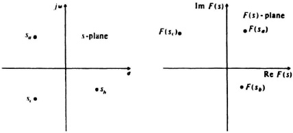
Figure 2.1   Mapping of a single-valued function from the s plane to the F(s) plane.

Figure 2.2   Mapping of a multivalued function from the s plane to the F(s) plane.

is analytic at every point in the s plane except at the points s = 0, −4 and −6. At these three points, the value of the function F(s) is infinity. However, the function

is analytic at every point in the s plane. Points in the s plane where the function F(s) is analytic are defined as ordinary points.

The derivative of an analytic function F(s) is given by

Because Δs = Δσ + jΔω, Δs can approach zero along an infinite number of different paths. If the derivative is taken along two specific paths, Δs = Δσ (parallel to the real axis) and Δs = jΔω (parallel to the imaginary axis) are equal, then the derivative is unique for any other path Δs = Δσ + jΔω and, therefore, the derivative exists.

To illustrate this, first let us consider the case where Δs = Δσ. Then,

Secondly, let us consider the path Δs = jΔω For this case,

Setting the values of these derivatives from Eqs. (2.5) and (2.6) equal to each other, we obtain the following:

Therefore, if the equations of

and

hold, then the derivative

is uniquely determined. Equations (2.8) and (2.9) are referred to as the Cauchy-Riema conditions and, if these conditions are satisfied, then the function F(s) is analytic.

As an example, let us analyze the following function:

Therefore,

where

Therefore,

and

Except for the condition of s = −4 (e.g., σ = −4 and ω = 0), F(s) satisfies the Cauchy–Riemann conditions:

Therefore, the function F(s) of Eq. (2.10) is analytic in the entire s plane except at s = −4(σ = −4, ω = 0).

We can obtain the derivative of the function F(s) from Eq. (2.10) at all points except at s = −4 from:

Derivatives of an analytic function such as F(s) of Eq. (2.10) can be determined simply by differentiating F(s) with respect to s:

B.  Singularities, Poles, and Zeros

Singularities are defined as points in the s plane where the function, or its derivatives, do not exist. An important example of a singularity is a pole. If a function F(s) is analytic in the region of s_j, except at the poles of s_j, then F(s) has a pole of order q (where q is finite) at s = s_j if

is finite. Therefore, the denominator of F(s) must contain the factor (s − s_j)^q, and the function becomes infinite when s = s_j. In Eq. (2.3), the function has a simple pole (i.e., poles of order one) at s = 0, −4, and −6. As a more complex example consider the function

This function has simple poles at s = 0, −4, and −10. In addition, it has a pole of order 2 at s = −20.

Finally, we consider the concept of zeros. If a function F(s) is analytic at s = s_j, then F(s) has a zero of order q (where q is finite) at s = s_j, if

is finite. Therefore, the numerator of F(s) must contain the factor (s − s_j)^q, and the function becomes zero where s = s_j. For example, in Eq. (2.20), there is a simple zero (i.e., a zero of order 1) at s = −1 and a zero of order 2 at s = −8.

Another important point to emphasize before leaving this discussion of poles and zeros is that the total number of poles has to equal the total number of zeros (including zeros at infinity) for functions that are defined to be the quotient of two polynomials in s. For example, in Eq. (2.20), we have five finite poles at s = 0, −4, −10, and a double pole at −20. We have three finite zeros: one at −1 and a double one at −8. However, there have to be two zeros at infinity because

We conclude from this that F(s) has a total of five zeros (three finite zeros and two infinite zeros) and five poles in the overall s plane.