3.5.  TRANSFER-FUNCTION AND STATE-VARIABLE REPRESENTATION OF TYPICAL HYDRAULIC DEVICES

Hydraulic components are commonly found in control systems that are either all hydraulic or a combination of electromechanical and hydraulic devices [6, 13]. The procedures used for deriving the transfer function representation of some commonly used hydraulic control system devices from their basic differential equations are illustrated in this section. We specifically consider hydraulic motors, pumps, and valves.

A.  Hydraulic Motor and Pump

There is no essential difference between a hydraulic pump and motor, just as there is no essential difference between a dc generator and a dc motor. Basically, the hydraulic device is classified as a motor if the input is hydraulic flow or pressure and the output is mechanical position; or a pump if the input is mechanical torque and the output is hydraulic flow or pressure.

Figure 3.21 illustrates a commonly used hydraulic power transmission system. This device, which is capable of controlling large torques, consists of a variable displacement pump that is driven at a constant speed. A control stroke, which determines the quantity of oil pumped, also controls the direction of fluid flow. The angular velocity of the hydraulic motor is proportional to the volumetric flow and is in the same direction as the oil flow from the pump. A functional diagram of the hydraulic transmission is illustrated in Figure 3.22.

The amount of oil displaced per revolution of the hydraulic pump is a function of the tilt angle θ_p(t). When θ_p(t) = 0°, there is no flow in the oil lines. As θ_p(t) is increased in the positive diretion, more oil flows in the lines with the direction shown. When θ_p(t) is negative, the direction of oil flow reverses.

In order to derive the differential equation relating θ_p(t) and θ_c(t), we must define certain hydraulic quantities. The volume of oil flowing from the pump, Q_p(t) is composed of flow of oil through the motor, Q_m(t), leakage flow around the motor, Q_l(t), and compressibility flow, Q_c(t) that is,

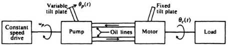
Figure 3.21  Hydraulic power transmission system.

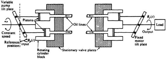
Figure 3.22  Functional block diagram of a hydraulic power transmission system.

It can be shown that

where

K_P = volumetric pump flow per second per angular displacement of θ_p(t)θ_p(t) = displacement of the pump stroke;

where

V_m = volumetric motor displacement
ω_c(t) = angular velocity of motor shaft:

where

L = leakage coefficient of complete system (ft³/sec)/(lb/ft²),
P_L(t) = load-induced pressure drop across motor (lb/ft²); and

where

V = total volume of liquid under compression (ft³)
K_B = bulk modulus of oil (lb/ft²).

Substituting Eqs. (3.124)–(3.127) into Eq. (3.123), we obtain the relationship

The torque available to drive the motor inertia is

Substituting Eq. (3.129) into (3.128), we obtain

The Laplace transform of Eq. (3.130) is given by

The transfer function of this device, defined as the ratio of the output θ_c(s) to the input θ_p(s), is given by

and its simple block diagram is illustrated in Figure 3.23. It is important to emphasize, however, that even a relatively small amount of air in the oil lines would lower K_B. This would cause the resonant frequency of the system to decrease sharply and reduce its capabilities. In addition, a large volume of oil in the lines between the hydraulic pump and motor has a similar effect. Therefore, these lines should be as short and narrow as possible.

Equation (3.132) can be written in differential-equation form as follows:

This third-order differential equation can be written as three first-order differential equations be defining

The resulting state equations are given by

In phase-variable canonical form, these equations become

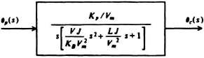
Figure 3.23.  Block diagram of a pump-controlled hydraulic transmission system.

where

B.  Hydraulic Valve-Controlled Motor

Another method of controlling a hydraulic motor is with a constant-pressure source and a valve that controls the flow of oil through it. A valve-controlled hydraulic system is usually smaller than a pump-controlled system and less efficient. Due to the increased losses the time constants are greatly reduced, and the speed of response is greater. Valve-controlled systems also have the disadvantages associated with devices whose characteristics are nonlinear.

Figure 3.24 illustrates a valve-controlled hydraulic system. A fluid source, at constant pressure, is provided at the center of the control valve. Fluid-return lines are located on each side of this pressure source. When the control valve is moved to the right, hydraulic fluid flows through line A into the hydraulic motor. This results in a pressure differential across the piston of the motor which causes it also to move to the right. This action caused fluid to be pushed back into the valve through line B which returns it to the sump through line E. Similar operation occurs when the control valve is moved to the left. Observe that all fluid flows are blocked when the control valve is in the neutral position, as shown in Figure 3.24.

Figure 3.25 represents the characteristics for the valve-controlled hydraulic motor. The pressure between lines going to the motor is denoted by P, the flow through these lines is denoted by Q, and r(t) denotes the displacement of the valve from its neutral position. Although these characteristics are nonlinear, it will be assumed that they are linear for small input displacements. This is basically an application for small-signal theory, used so frequently by circuit designers. For small excursions from a given quiescent operating point,

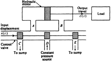
Figure 3.24  A valve-controlled hydraulic system.

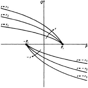
Figure 3.25  Valve characteristics.

Figure 3.26  Block diagram of a valve-controlled hydraulic transmission system.

At any given quiescent operating point, it will be assumed that ∂Q/∂P and ∂Q/∂r are constants.

The transfer function relating the input r(t) and output c(t) can be obtained by comparing the valve-controlled hydraulic system with the pump-controlled hydraulic system. Studying these two systems carefully, it is observed that ΔQ is analogous to Q_p, M (moment of inertia) is analogous to J, ΔP is analogous to P_L, and Δr is analogous to θ_p(t). Using these analogies, the transfer function can easily be found to be given by

The term L – ∂Q/∂P in the denominator of this equation is always positive, because Figure 3.25 indicates that ∂Q/∂P is always negative. The simple block diagram for this system is illustrated in Figure 3.26. It is left as an exercise to the reader to determine what the transfer function of the system is if a spring and damper are attached to the control rod (see Problem 3.11), and to determine the state-variable vector form of Eq. (3.143).