5.10.  ILLUSTRATIVE PROBLEMS AND SOLUTIONS

This section provides a set of illustrative problems and their solutions to supplement the material presented in Chapter 5.

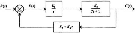
Figure I5.1

I5.l. The control system of Figure I5.1 contains position and rate feedback:

(a)  Determine the closed-loop transfer function C(s)/R(s).

(b)  Determine the sensitivity of the closed-loop transfer function to K₂ as a function of s.

(c)  Determine the sensitivity of the closed-loop transfer function to K₂ at dc.

SOLUTION:(a)

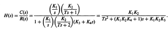
(b)

where

Therefore,

(c)

I5.2. The sensitivity of the following control systems is to be analyzed:

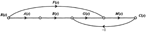
Figure I5.2

(a)  Determine the overall transfer function, H = C(s)/R(s).

(b)  Determine the sensitivity of the control system’s transfer function, H(s) = C(s)/R(s) with respect to the transfer function M(s).

(c)  Determine the sensitivity of the control system’s transfer function, H(s) = C(s)/R(s) with respect to the transfer function B(s).

(d)  What happens to your results in part (c) if the transfer function A(s)G(s)B(s) is much greater than F(s)?

SOLUTION:(a)

(b)

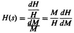
where

.

Therefore,

.

(c)

where

.

Therefore,

.

(d)  For A(s)G(s)B(s) much greater than F(s), then

I5.3. A control-system engineer is designing a feedback amplifier using two stages of gain. He is not certain which of the following two systems will result in a smaller sensitivity to the amplifier gain, K_a:

Figure I5.3

(a)  Determine the closed-loop transfer functions, C(s)/R(s), for each design, assuming that K_a = K_b = 50.

(b)  Compare the sensitivities of the two systems with respect to the amplifier gain K_a.

(c)  Why do the results come out of the way they do, and which design would you select?

SOLUTION: (a) For System No. I:

For System No. II:

Therefore, H_II(s) = 50.

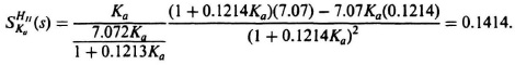
(b)  For System No. I:

For System No. II:

and

Therefore,

(c)

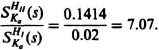
The sensitivity of System No. 1 is less than that of System No. 2 because System No. 1 has feedback around both K_a and K_b, with the result that the gain of System No. 1, H(s), is 50. The gain around K_a in System No. II is only 7.07. Therefore, the sensitivity of Hs) to variations in K_a in System No. I is less than that in System No. II.

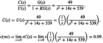
I5.4. The accuracy of the following control system is to be analyzed:

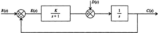
Figure I5.4

(a)  Determine the steady-state error, e_ss, for a unit step input, r(t) = U(t) with K = 10.

(b)  Determine the steady-state error, e_ss, for a unit disturbance step input, d(t) = U(t) with K = 10.

(c)  Determine the value of K so that the resulting steady-state error due to a disturbance step input, d(t) = U(T) equals 5% of the disturbance step input value.

SOLUTION: (a) Since the forward transfer function, C(s)/E(s), has one pure integrator in it, the steady-state error, e_ss, equals 0.

(b)

Therefore,

(c)

Therefore,

Therefore, K = 20.

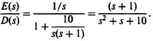
I5.5. The control system of a radar-controlled anti-aircraft gun is to be designed. In the illustration shown, the tracking radar measures the distance d to the crossing target aircraft, and the angle of the antenna with respect to the ground, θ_r.

Figure I5.5(I)

For the design of the control system, assume the crossing target aircraft speed is 1500 ft/sec at a range of 25000 ft, and it is assumed to be perpendicular to the line-of-sight from the radar. The following control system for positioning the gun is to be analyzed:

Figure 15.5(II)

(a)  Determine the angular velocity, in rad/sec, the radar sees due to the crossing target.

(b)  The maximum desired miss distance of a shell fired from the anti-aircraft gun is 2 ft. How does this translate to an angular steady-state-error, e_ss, in radians for the control system?

(c)  Determine the velocity constant, K_v, needed from the control sysem to satisfy the answers found in parts (a) and (b).

(d)  Determine the value of the amplifier gain. K, in the control system to achieve the velocity constant, K_v, found in part (c).

SOLUTION: (a) The problem can be analyzed from the following:

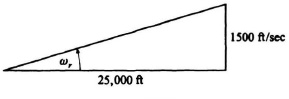
Figure I5.5(III)

Therefore,

(b)  The problem can be analyzed from the following:

Figure I5.5(iv)

Therefore,

(c)

Therefore, from the answers in parts (a) and (b), we obtain the following:

0.00008 =

Therefore,

K_v = 750.

(d)  Using the answer from part (c), we obtain the following:

Therefore,

and

k = 1125.

I5.6. Determine the values of K and b for the control system shown in order that the damping ratio of the system is 0.5, and the settling time of the unit-step response is 0.2 sec.

Figure I5.6

SOLUTION: (a) Using Mason’s Theorem, we obtain the following:

Simplifying this equation, we obtain the following:

From Eq. (5.41),

Substituting into this equation for t_s,

Therefore,

ζω_n = 20.

We also know from comparing the denominator of Eq. (4.3) and that of C(s)/R(s),

2ζω_n = 2.5 + 25 b.

Therefore, b = 1.5.

Since the problem states that the damping ratio, ζ = 0.5, and since we determined that ζω_n = 20, we can solve for ω_n as follows:

0.5ω_n = 20.

Therefore, ω_n = 40. We can now determine K by comparing the equation for C(s)/R(s) and Eq. (4.3):

Substituting for ω_n = 40, we solve for K:

40² = 6.25K.

Therefore, K = 256.

I5.7. The steering control system of a large ship represents a feedback control system as illustrated in the block diagram shown. The function of the ship’s rudder is to compensate for the ship’s deviation from its desired heading due to sea waves and wind disturbances (where the ship acts as a sail when wind strikes it).

Figure I5.7

(a)  Find the steady-state value of the output due to a constant sea wave and wind disturbance which can be approximated as a unit step: U(s) = 1/s. Assume that the rudder input is zero: R(s) = 0.

(b)  Determine the value that the ship’s steering officer should set the rudder, R(s), to compensate for the disturbance in part (a).

SOLUTION:(a)

(b)

Therefore, for C(s) = 0, it is necessary that we design

U(s) + KR(s) = 0

Or,

Therefore,

r(t) = −0.1 U(t).

I5.8. A control system containing a reference input R(s) and a disturbance D(s) is represented by the following block diagram:

Assuming that the system is stable, determine the following:

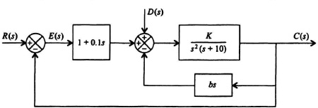
Figure I5.8

(a)  The transfer function C(s)/E(s) which represents the transfer function of the control system with the outer loop opened.

(b)  The steady-state error of the system in terms of K and b for a unit-ramp input, r(t) = tU(t). Assume that D(s) = 0 in this part.

(c)  The steady-state value of c(t) when D(s) = 1/s, a unit step input. Assume that R(s) = 0 in this part.

SOLUTION:

(a)

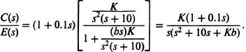
(b)

Therefore,

(c)

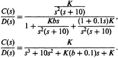
For D(s) = 1/s, we obtain the following expression for C(s):

I5.9. We wish to analyze the second-order control system illustrated in Figure 4.1, whose closed-loop transfer function was developed in Eq. (5.53). Assuming that T_m = 1 sec, what should K_m be designed to be so that the ITAE criterion is achieved for this zero steady-state step error system?

SOLUTION: From Eq. (5.53) with T_m = 1, we obtain the following

From Table 5.5, the ITAE form for a second-order control system is given by:

Setting like coefficients equal to each other from these two equations, we obtain the following:

1.4ω_n = 1

and

Solving these two simultaneous equations, we obtain the following:

ω_n = 0.71

and

K_m = 0.51.

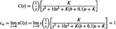
I5.10. We wish to analyze the control system illustrated in Figure 5.9, which contains two pure integrations and whose closed-loop transfer function was given in Eq. (5.55). Assuing that T₂ = 1, determine the value sof K and T₁ so that the ITAE criterion is achieved for this zero steady-state ramp error system.

SOLUTION: From Eq. (5.55) with T₂ = 1, we obtain the following:

From Table 5.6, the ITAE form for a third-order control system is

Setting like coefficients equal to each other from these two equations, we obtain the following:

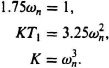
Solving these three equations simultaneously, we obtain:

ω_n = 0.571
K = 0.186,
T₁ = 5.697.