PROBLEMS

5.1. Assume that the system shown in Figure P5.1 has the following characteristics:

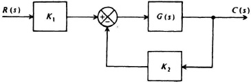
Figure P5.1

K₁ = 10 V/rad,
K₂ = 10 V/rad,
G(s) =

(a)  Determine the sensitivity of the system’s transfer function H(s) with respect to the input transducer, K₁.

(b)  Determine the sensitivity of the system’s transfer function H(s) with respect to the feedback transducer, K₂.

(c)  Determine the sensitivity of the system’s transfer function H(s) with respect to G(s)

(d)  Indicate qualitatively the frequency dependency of

5.2. For the system in Figure P5.2, assume the following characteristics:

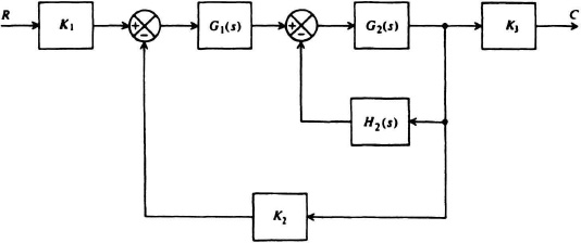
Figure P5.2

(a)  Determine the sensitivity of the system’s transfer function H(s) with respect to G₁(s) at ω = 1 rad/sec.

(b)  Determine the sensitivity of the system’s transfer function H(s) with respect to G₂(s) at ω = 1 rad/sec.

(c)  Determine the sensitivity of the system’s transfer function H(s) with respect to H₂(s) at ω = 1 rad/sec.

(d)  Determine the sensitivity of the system’s transfer function H(s) with respect to K₃ at ω = 1 rad/sec.

(e)  List the answers of parts (a)–(d) in tabular form with the lowest value first and the largest value last for ω = 1 rad/sec. Normalize your table with repect to the lowest sensitivity found. How could this table change for a different choice of frequency?

5.3. Figure P5.3a illustrates the block diagram of a computer-controlled machine tool that utilizes a position loop and a correction loop [5]. A practical problem in machine-tool application is the fact that the desired tool position is ordinarily fed back by the position loop as shown, but this is not indicative of the condition and shape of the finished part. In reality, the finished part is ordinarily removed from the feedback effect due to the tool–work interface. Because these effects are complex and difficult to predict, the process output will not conform precisely to that desired. By means of the correction loop, information is obtained from the process output by means of sensors coupled as closely as possible to the tool–work interface. These sensor signals, which represent variables such as torque, vibration, and temperature, are fed back to improve the performance of the machine tool control system. Figure P5.3b illustrates an equivalent block-diagram representation.

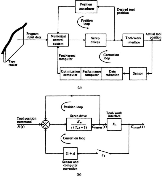
Figure P5.3

(a)  With switch S₁ open and the correction loop inoperative, determine the sensitivity of the system’s transfer function T(s) to variations of K_m, T_m, and K₁.

(b)  Repeat part (a) with switch S₁ closed and the correction loop operative.

(c)  What conclusions can you draw from your results?

5.4. For the system illustrated in Figure P5.4 assume the transfer functions indicated.

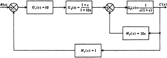
Figure P5.4

(a)  Determine the sensitivity of the system’s transfer function with respect to G₁(s).

(b)  Determine the sensitivity of the system’s transfer function with respect to G₃(s).

(c)  Determine the sensitivity of the system’s transfer function with respect to H₃(s).

(d)  Determine the sensitivity of the system’s transfer function with respect to H₁(s).

(e)  List the answers of parts (a)–(d) in tabular form with the lowest value of sensitivity first and the largest value last at a frequency of 1 rad/sec. Normalize your table with respect to the lowest sensitivity found. How could this table change for a different choice of frequency?

5.5. Simulators for training pilots of commercial and military aircraft are receiving greater emphasis and attention. A simulator used for training the pilot of a new aircraft is to be designed. This simulator will have a three-degree-of-freedom capability (roll, pitch, yaw), which will give the trainees a “feel” of the dynamics that the pilots will experience during flight operation. The controls and interior of the cockpit will be designed to be a very close replica of the actual aircraft, to give the pilot a real-world feel of the aircraft—both esthetically and dynamically. For purposes of this analysis, assume that the pitch loop can be represented by the block diagram in Figure P5.5.

Figure P5.5

(a)  Determine the sensitivity of the pitch loop’s transfer function, H(s), to the amplifier gain, K_a, in terms of the system parameters.

(b)  Determine the sensitivity of the pitch loop’s transfer function to the feedback transducer, H₁, in terms of the system parameters.

(c)  For the flight environment expected to be encountered, parameter variations at ω = 1 rad/sec are very critical. Determine the absolute values of these two sensitivities at this frequency.

(d)  What conclusions can you reach from your results?

5.6. The time constant of a two-phase ac servomotor is not a precise parameter, and is subject to change caused by aging and environmental conditions such as temperature changes. The control system in Figure P5.6 containing a two-phase ac servomotor, is to be analyzed for its sensitivity to the two-phase ac servomotor’s time constant, T.

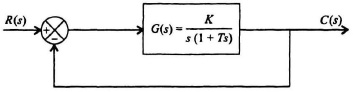
Figure P5.6

Determine the sensitivity of the control system’s transfer function, H(s) = C(s)R(s), with respect to the time constant T.

5.7. The signal-flow graph representation of the control system in Figure P5.7 is to be analyzed.

(a)  Determine the overall transfer function C(s)/R(s).

(b)  The selection of G₄(s) is critical. Determine the sensitivity .

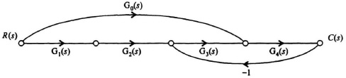
Figure P5.7

5.8. The block diagram for the control system that positions an aircraft’s rudder is shown in Figure P5.8.

Figure P5.8

(a)  What is the sensitivity of the system transfer function, C(s)/R(s), to small changes in K_a? Express your answer for as a function of s.

(b)  Determine the magnitude of the sensitivity at wind gust disturbances which can be approximated to exist at ω = 1 rad/sec. Assume that K_a = 10.

(c)  Determine the magnitude of the sensitivity when the aircraft breaks the sound barrier, and the sonic boom causes a vibration frequency disturbance which can be approximated at ω = 1000 rad/sec. Assume that K_a = 10.

(d)  What conclusions can you reach from your results?

5.9. In the control system illustrated in Figure P5.9, attention is to be focused on the quality of components to be specified for it. Determine the sensitivity of the system’s transfer function, H(s) = C(s)/R(s) with respect to the following system parameters:

Figure P5.9

(a)  A(s)

(b)  G(s)

(c)  H′(s)

In each case, evaluate the sensitivity function, and then determine its absolute value at ω = 1 rad/sec.

5.10. The sensitivity of the feedback control system illustrated in Figure P5.10 is to be determined.

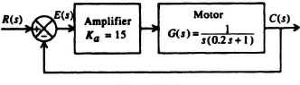
Figure P5.10

(a)  Determine the system’s transfer function H(s) = C(s)/R(s).

(b)  Determine the sensitivity of H(s) with respect to the motor G(s). Show your answer in its simplest possible form as a function of s.

(c)  What is the absolute value of the sensitivity of H(s) with respect to G(s) at ω = 1 rad/sec?

(d)  If the value of the motor’s transfer function G(s) varies by ±25%, by how much will the system’s transfer function H(s) vary at ω = 1 rad/sec?

5.11. A control system is used to position the rudder of an aircraft. Its block diagram can be adequately represented as shown in Figure P5.11.

Figure P5.11

(a)  Determine the sensitivity of the system’s transfer function with respect to G(s).

(b)  Determine the sensitivity of the system’s transfer function with respect to K_a.

(c)  Determine the absolute value of the sensitivities determined in parts (a) and (b) to wind gusts that can be approximated to primarily exist at 1 rad/sec. Which element is more sensitive at this frequency, the amplifier or servo motor?

(d)  How much will the system’s transfer function vary at 1 rad/sec if K_a changes by 50%?

5.12. A control-system engineer wants to determine the quality of a tachometer needed to be specified in the control system shownin Figure P5.12, which uses both position and rate feedback. In making the decision, it is known that the control system must follow an input at R(s), the dominant frequency component of which is at 0.5 rad/sec.

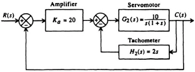
Figure P5.12

(a)  Determine the sensitivity of the system’s transfer function H(s) with respect to H₂(s) in terms of the Laplace transform s.

(b)  Determine the absolute value of this sensitivity at a frequency of 0.5 rad/sec.

(c)  What decision regarding the quality of the tachometer should be made?

5.13. Automatic control theory can also be applied to automatic warehousing and inventory control systems [6]. Of particular importance in these systems is the smooth flow of material. Figure P5.13 illustrates a block diagram that is representative of this class of control systems.

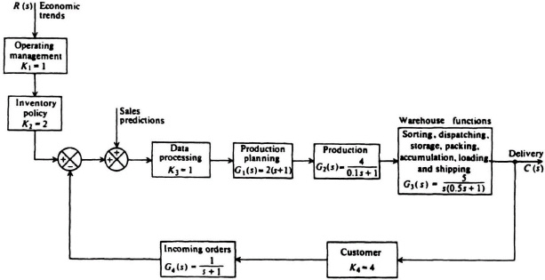
Figure P5.13

(a)  Determine the sensitivity of the system’s transfer function C(s)/R(s) with respect to production planning. G₁(s).

(b)  Determine the sensitivity of the system’s transfer function with respect to production, G₂(s).

(c)  Determine the sensitivity of the system’s transfer function with respect to the various warehouse functions G₃(s).

(d)  Determine the sensitivity of the system’s transfer function with respect to incoming orders, G₄ (s).

(e)  Determine the sensitivity of the system’s transfer function with respect to the inventory policy, K₂.

(f)  For which two parameters is the system most sensitive, and what conclusions can you reach from your results?

(g)  Indicate qualitatively the frequency dependence of the sensitivity functions.

5.14. Figure P5.14 illustrates an electronic pacemaker used to regulate the speed of the human heart. Assume that the transfer function of the pacemaker is given by G_p(s) = K/(0.05s + 1) and assume that the heart acts as a pure integrator.

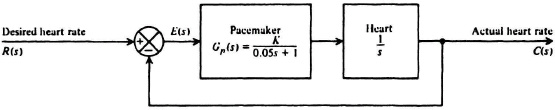
Figure P5.14

(a)  For optimum response, a closed-loop damping ratio of 0.5 is desired. Determine the required gain K of the pacemaker in order to achieve this.

(b)  What is the sensitivity of the system transfer function. C(s)/R(s), to small changes in K?

(c)  Determine this sensitivity at dc.

(d)  Find the magnitude of this sensitivity at the normal heart rate of 60 beats/minute.

5.15. A control system used to position a load is shown in Figure P5.15.

Figure P5.15

(a)  Determine the steady-state error for a step input of 10 units.

(b)  How should G(s) be modified in order to reduce this steady-state error to zero?

5.16. A unity feedback control system has a forward transfer function given by

Determine the steady-state error for an input given by

r(t) = (4 + 6t + 3t²)U(t).

5.17. The block diagram of a simple instrument servomechanism is shown in Figure P5.17.

Figure P5.17

(a)  Determine the steady-state error resulting from the input of a ramp that may be represented by

r(t) = (10t)U(t).

(b)  Determine the steady-state error resulting from the following input:

r(t) = (4 + 6t + 3t²)U(t).

5.18. Repeat Problem 5.17 with the transfer function of the system given by

5.19. A ground-based tracking radar is used to track aircraft targets very precisely. The block diagram of the azimuth axis of the tracking radar can be adequately represented by the block diagram of Figure P5.19.

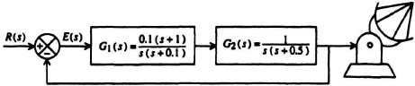
Figure P5.19

Determine the steady-state errors of the tracker for the following types of inputs caused by the aircraft dynamics:

(a)  r(t) = (10t)U(t).

(b)  r(t) = (10t + 6t²)U(t).

5.20. A control system containing a reference input, R(s), and a disturbance input, D(s), is illustrated:

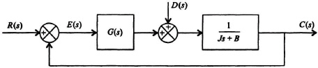
Figure P5.20

(a)  Determine the steady-state error, e_ss for a unit-step disturbance at D(s) in terms of the unknown transfer function G(s).

(b)  Select the simplest value of G(s) which will result in zero steady-state error for E(s) when D(s) is a unit step input.

5.21. The block diagram of a control system containing a disturbance, D(s), is illustrated in Figure P5.21.

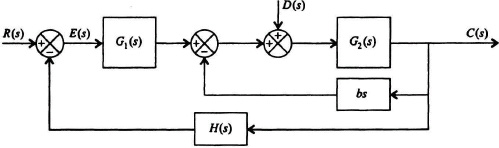
Figure P5.21

(a)  Determine the transfer function, E(s)/D(s).

(b)  Determine the steady-state error for E(s) when D(s) is a unit step input assuming that H(s) = b = 1, and that G₂(s) = 1/(s + 1), in terms of the unknown transfer function, G₁ (s).

(c)  Select the simplest value of G₁(s) which will result in zero steady-state error for E(s) when D(s) is a unit step input.

5.22. We wish to determine the accuracy of the control system illustrated in Figure P5.22.

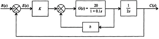
Figure P5.22

Assuming that the system is stable, determine the following:

(a)  The transfer function, C(s)/E(s) which represents the open-loop transfer function of the control system with the outer loop opened. Reduce your answer to its simplest form.

(b)  The steady-state error, e_ss, for r(t) = U(t).

(c)  The steady-state error, e_ss for r(t) = tU(t).

(d)  The steady-state error, e_ss for r(t) = (t²/2)U(t).

(e)  Assuming that b = 1, what must K be designed for in order that the steady-state error, e_ss, equals 0.1 when r(t) = tU(t).

5.23. The block diagram of a control system containing a disturbance, D(s), is illustrated in Figure P5.23.

Figure P5.23

The process to be controlled is represented by G(s), and G₀(s) and H(s) represent the controller transfer function.

(a)  Determine the transfer function, C(s)/R(s).

(b)  Determine the transfer function C(s)/D(s).

(c)  Determine C(s)/R(s) when G₀(s) = G(s), assuming D(s) = 0.

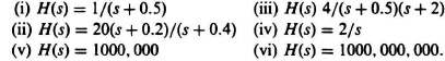
(d)  Assuming that

select H(s) from the following choices so that when D(s) = 1/s and R(s) = 0, the steady-state value of c(t) is equal to zero:

5.24. We know from Eq. (5.37) that the steady-state error of a second-order control system to a unit ramp input is given by 2ζ/ω_n (reciprocal of the velocity constant, K_υ). This steady-state error to a unit ramp input can be eliminated if the input, R(s), is introduced into the system through a proportional-plus-derivative filter, as illustrated in Figure P5.24, and the value of A is properly designed.

Figure P5.24

Determine the value of A which will result in zero steady-state error to a unit ramp input at the input, R(s), assuming that the error, e(t), is defined as

e(t) = r(t) − c(t).

5.25. For the system whose block diagram is shown in Figure P5.25, determine the following:

Figure P5.25

(a)  Steady-state error resulting from an imput of r(t) = (100t)U(t).

(b)  Steady-state error resulting from an input of r(t) = (12t²)U(t).

(c)  Steady-state error resulting from an input of r(t) = (20+ 100t + 12t²)U(t).

5.26. For the control system shown in Figure P5.26, determine the steady-state error e(t) resulting from the application of the following inputs:

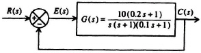
Figure P5.26

(a)  r(t) = (10t)U(t).

(b)  r(t) = (2 + 4t + 6t²)U(t).

(c)  How would you modify G(s) to reduce the steady-state error in part (b) to zero?

5.27. For the system shown in Figure P5.27, determine the following:

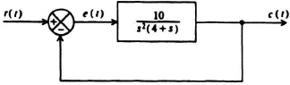
Figure P5.27

(a)  Steady-state error resulting from an input

r(t) = (10t)U(t).

(b)  Steady-state error resulting from an input

r(t) = (4 + 6t + 3t²)U(t).

(c)  Steady-state error resulting from an input

r(t) = (4 + 6t + 3t² + 1.8t³)U(t).

5.28. Repeat Problem 5.27 with the transfer function of the system given by

5.29 A common problem in the television industry is that of picture wobbling or jumping because of movement of the TV camera while a picture is being taken. The effect of this problem is easily understood by examining Figures P5.29a and P5.29b. When the camera is at rest (as illustrated in Figure P5.29a) a light ray entering the camera lens impinges on point A within the camera. However, if the camera is jolted upward through an angle δ (as in Figure P5.29b, the light ray is displaced from its original location at point A to point B. This can be corrected by means of the system illustrated in Figure P5.29b. The concept utilizes a device that changes the shape of a fluid lens such that the ray’s impinging point does not move [7]. The front transparent plate is rotated in the vertical plane by a torque motor. The rear plate is rotated in the horizontal plane. Two rate gyros are mounted in the camera to detect any disturbances. Their output is fed to a servo amplifier that adjusts the driving current to the torque motors. Tachometers close the rate feedback loops. The equivalent block diagram of one such axis is illustrated in Figure P5.29c. Observe that the feedback loop uses speed from the rate gyro as the reference input and speed from the tachometer to indicate speed of the bellows.

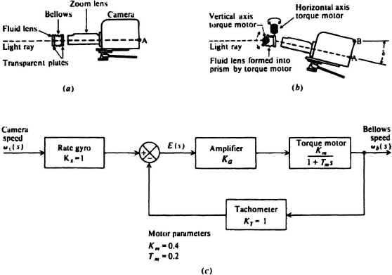
Figure P5.29 (Reprinted from Control Engineering, May 1965 © 1965 by Cahners Publishing Company)

(a)  Determine the required value of amplifier gain K_a in order that the steady-state error resulting from a camera scanning speed of 50°/sec is only 1°/sec.

(b)  What is the steady-state error of this system resulting from camera accelerations of any magnitude?

5.30 A servomechanism, shown in Figure P5.30, is used to drive an inertia load through gearing of negligible inertia.

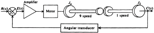
Figure P5.30

1.  ac motor characteristics: Torque-speed slope = 4.5 × 10⁻⁶ lb ft/(rad/sec). Stall torque constant = 8.5 × 10⁻⁶ (lb ft)/V.

2.  Load inertia= J_L = 40 × 10⁻⁶ lb ft sec² (assume J_mN² ≪ J_L).

3.  Amplifier gain = 10.

4.  Gear ratio = 9:1 (steps motor speed down).

5.  Angular transducer transfer function = 1.

(a)  What is the transfer function G(s) relating C(s) and E(s) of the system?

(b)  What are the undamped natural frequency ω_n and the damping ratio ζ?

(c)  What is the percent overshoot and time to peak resulting from the application of a unit step input?

(d)  What is the steady-state error resulting from application of a unit step input?

(e)  What is the steady-state error resulting from application of a unit ramp input?

(f)  What is the steady-state error resulting from application of a parabolic input?

5.31. Repeat Problem 5.30 with the assumption that the motor inertia J_m is 1.11 × 10⁻⁶ lb ft sec².

5.32. Repeat Problem 5.30 with the amplifier’s gain increased to 100.

5.33. Automatically controlled machine tools form an important aspect of control-system application. The major trend has been towards the use of automatic numerically controlled machine tools using tape inputs [8]. The justification of using tape has been the elimination of costly contour templates and the reduction of the machine set-up procedure required. In addition, it eliminates the tedium of repetitive operations required of human operators, and the possibility of human error. Figure P5.33 illustrates the block diagram of an automatic numerically controlled machine-tool position control system, using a punched tape reader, to supply the reference signal.

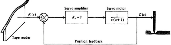
Figure P5.33

(a)  What are the undamped natural frequency ω_n and damping ratio ζ?

(b)  What are the percent overshoot and time to peak resulting from the application of a unit step input?

(c)  What is the steady-state error resulting from the application of a unit step input?

(d)  What is the steady-state error resulting from the application of a unit ramp input?

5.34. The transient response of the control system in Figure P5.34 is to be analyzed.

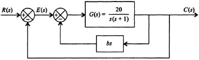
Figure P5.34

(a)  Determine C(s)/R(s).

(b)  Determine the rate feedback constant b so that this control system has a damping ratio of 0.7.

(c)  Determine the rise time, t_r.

(d)  Determine the time to peak, t_p.

(e)  Determine the settling time, t_s.

5.35. The transfer function of a closed-loop control system is given by

Based on test data, it has been determined that the system exhibits a position constant K_p of 8. Determine the value of the unknown zero z.

5.36. Modem ocean-going ships utilize stabilization techniques in order to minimize the effects of oscillations due to waves. By utilizing hydrofoils or fins, stabilizing torques can be generated in order to stabilize the ship [9]. Figure P5.36a illustrates this concept employing stabilizing fins. An equivalent block diagram of the system is illustrated in Figure P5.36b. The reference input signal, θ_desired, is normally set equal to zero. A vertical gyro, which senses deviations from θ = 0, feeds back a correction signal that activates the fins in order to drive the error signal to zero. The disturbance signal U(s) represents the disturbance torque due to the waves.

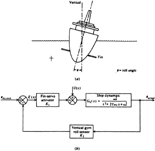
Figure P5.36

(a)  Determine the effect of the disturbance torque U(s) on system error E(s) if it is assumed that K₁K₂G_s(s) ≫ 1. What conclusions can you draw from your result?

(b)  Based on the approximation of part (a), what should K₁ be set at in order to reduce a disturbance torque input at U(s) of 10° to an equivalent system steady-state error of 0.1 °?

5.37. As digital computers become more common in every phase of industry and the scientific communities, there is an ever-increasing demand for the storage and speedy retrieval of data [10]. The resulting control-system requirements are usually quite stringent and usually require new techniques. Figure P5.37a illustrates a system used to control the position of the read/write heads in a random-access magnetic-drum memory system [10]. The particular application had 64 data heads mounted in vertical pairs at 2-in intervals along a “head bar.” Although the controlling action is obtained by utilizing digital components, an equivalent representation of the control system is given in Figure P5.37b.

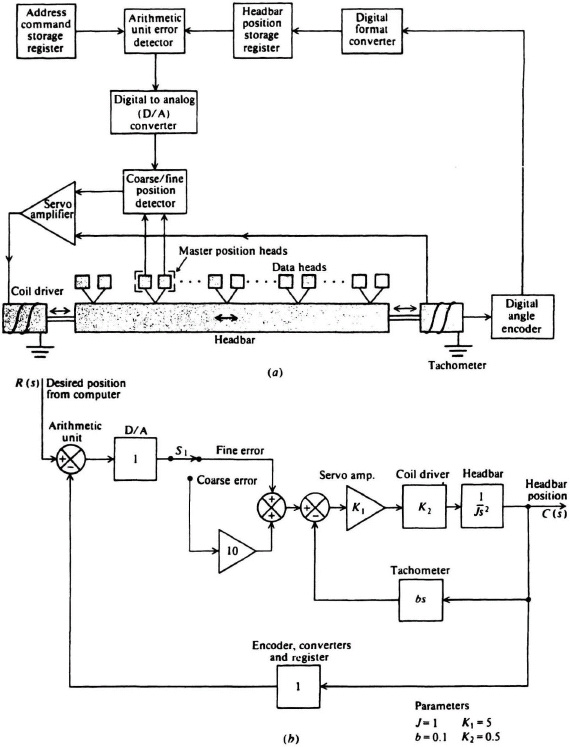
Figure P5.37

The headbar is free to move longitudinally. It is located between two magnetic drums whose axes of rotation are parallel with the longitudinal axis of the headbar. Each of the data heads in this system has access to a total of 200 tracks. The track accessed depends on the placement of the headbar within the limits of its 2-in travel. A fine and a coarse positioning loop are used to obtain the desired accuracy. An electronic switch S₁ switches the system so that it has a large amount of gain for large errors so that the system responds rapidly. For this condition, a large amount of overshoot is tolerated in order to achieve a fast rise time. For small errors, the fine system is activated which has a larger damping ratio, smaller overshoot, and a somewhat longer response time. Assume that the system switches when e(t) = 0.1 unit.

(a)  Determine the undamped natural frequency, damping ratio, overshoot, and time to peak for the “coarse” loop.

(b)  Repeat part (a) for the “fine” loop.

(c)  Determine the error of the coarse and fine loops to a unit step input.

(d)  Determine the error of the coarse and fine loops to a unit ramp input.

(e)  Determine the error of the coarse and fine loops to a unit parabolic input.

5.38. A fourth-order feedback system is illustrated in Figure P5.38. In order to satisfy the IT AE criterion, determine the values of K₁, β₁, and β₂ for a zero steady-state step error system.

Figure P5.38

5.39. Determine the values of K₁, K₂, ω_n and b, in the feedback system illustrated in Figure P5.39 which will satisfy the ITAE criterion for a zero steady-state step error system.

Figure P5.39

5.40. Repeat Problem 5.39 with the acceleration feedback element attentuated by a factor of 0.5. What conclusions can you draw from your result?

5.41. Repeat Problem 5.39 if the gain of the acceleration feedback element is doubled. What conclusions can you draw from your result?

5.42. A position-following system which can respond to position and ramp inputs with zero steady-state errors is shown in Figure P5.42. Determine the values of K_a and T that will satisfy the ITAE criterion for a zero steady-state ramp error system.

Figure P5.42

5.43. Robots are being used to a great extent in automating arc welding processes in manufacturing. This is especially true in the manufacture of automobiles. Figure P5.43 shows a photograph of the GMFanuc Robotics Corporation GMF ARC Mate Sr™ six-axis robot designed specifically for automating arc welding processes in a cost-effective manner. It uses ac servomotors that are brushless, which eliminates brush-related maintenance. A digital servo system enables high-speed movement, shorter positioning time, and improved path accuracy [11].

Figure P5.43 (a) Photograph of the GMFanuc Robotics Corporation GMF ARC Mate Sr.™ six-axis robot designed specifically for automating arc welding processes in a cost-effective manner. (Courtesy of GMFanuc Robotics Corporation) (b) Block diagram.

Let us assume that we have to design a robot such as this one, but it will be based on a continuous design and not on digital techniques, which are discussed in Chapter 9. It is also assumed that one of the axes can be represented by the block diagram shown in Figure P5.43b. For the purposes of our application, a critically damped system will be assumed to be desirable.

(a)  Determine the amplifier gain K_a so that the robot is criticaly damped in this axis.

(b)  Find the sensitivity function of the robot’s transfer function due to amplifier variations, , where H(s) = θ_out (s)/θ_in(s). Express the sensitivity as a function of s.

(c)  Determine the absolute value of the sensitivity at dc.

(d)  Determine the steady-state error for an input command signal of

r(t) = (4 + 6t)U(t).

5.44 The accuracy of the following control system is to be analyzed:

Figure P5.44

(a)  Determine the steady-state error, e_ss, for a unit step input, r(t) = U(t) with K = 10.

(b)  Determine the steady-state error, e_ss, for a unit disturbance step input, d(t) = U(t) with K = 10.

(c)  Determine the value of K so that the resulting steady-state error due to a disturbance step input, d(t) = U(T) equals 5% of the disturbance step input value.

5.45 We wish to analyze the second-order control system illustrated in Figure 4.1, whose closed-loop transfer function was developed in Eq. (5.53). Assuming that T_m = 2 seconds, what should K_m be designed for so that the ITAE criterion is achieved for this zero steady-state step error system?