8.6.  ACKERMANN’S FORMULA FOR DESIGN USING POLE PLACEMENT [5–7]

In addition to the method of matching the coefficients of the desired characteristic equation with the coefficients of det (sI − P_h) as given by Eq (8.19), Ackermann has developed a competing method. The pole placement method using the matching of coefficients of the desired characteristic equation with the coefficients of Eq (8.19) is very useful for control systems which are represented in phase-variable form, where phase variable refers to systems where each subsequent state variable is defined as the derivative of the previous state variable. Some control systems require feedback from state variables which are not phase variables. Such high-order control systems can lead to very complex calculations for the feedback gains. Ackermann’s method simplifies this problem by transforming the control system to phase variables, determining the feedback gains, and transforming the designed control system back to its original state-variable representation.

Let us represent a control system which is not represented in phase-variable form by the following:

We will assume that the controllability matrix [see Eq (8.65)] can be represented by

Subscript y is used to designate the original, non-phase-variable, controllability matrix. We will next assume that the control system can be transformed into the phase-variable representation using the following transformation:

Substituting Eq (8.79) into Eq (8.76) and Eq (8.77), we obtain:

Using the transformation of Eq (8.79), the controllability matrix for the transformed system defined by Eqs. (8.80) and (8.81) is:

The subscript x is used to designate the phase-variable form of the transformed control system. Equation (8.82) can be simplified to

Therefore, substituting Eq (8.78) into Eq (8.83), we find that

The transformation matrix A can be found from

Therefore, the transformation matrix A can be determined from the controllability matrices defined by Eq (8.65) and (8.83). Once the control system is transformed to the phase-variable form, the feedback gains h can be determined as described in Section 8.2.

Returning to Eq (8.4) to represent u(t) for the control system in phase-variable form,

the following is obtained by substituting Eq (8.86) into Eq (8.80):

Equation (8.87) can be simplified to the following phase-variable state equation:

The output equation remains as shown in Eq (8.81):

Because Eqs. (8.88) and (8.89) are in phase-variable form, the rules for pole placement developed in Section 8.2 for phase-variable systems are valid for this representation. We now have to transform Eqs. (8.88) and (8.89) back to the original state and output equation representation by using the transformation provided by Eq (8.79):

Substituting Eq (8.90) into Eq (8.88), we obtain the following:

Therefore, Eq (8.91) reduces to the following state equation:

The output equation is found by substituting Eq (8.79) in Eq (8.89):

By comparing Eq (8.92) with Eqs. (8.8) and (8.10), we find that the state-variable feedback constants for the original system are

A.  Example Applying Ackermann’s Formula for Design using Pole Placement

We wish to apply the pole placement concepts using Ackermann’s design formula to a system that uses linear-state-variable feedback. The system specifications require an overshoot of 4.33% and a settling time of 6 sec. The process transfer function is

and the control system’s signal-flow graph is given in Figure 8.16.

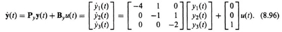
The state equation for the process illustrated in Figure 8.16 is:

Since we are going to need the controllability matrix D_y to convert this original system to phase-variable form [see Eq (8.85)], let us compute this controllability matrix for this original system:

The value of the determinant of D_y is −1, it is nonsingular, and the original control system is controllable as expected from inspection of Figure 8.16.

The next step is to transform the original system to the phase-variable form. This can easily be obtained from the transfer function C(s)/U(s), which can be determined from Figure 8.16:

Eq (8.98) can be reduced to the following [as stated in Eq (8.95)]:

We can determine the phase-variable state equations which represent the transfer function given by Eq (8.99). Defining x₁(t) = c(t), x₂(t) = (t), and x₃(t) = (t), we obtain the following:

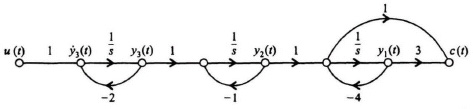
Figure 8.16  Signal-flow graph representation of process whose transfer function is defined in Eq (8.95).

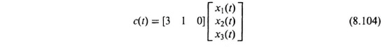
Therefore, the state and output equations in matrix vector form of the phase-variable control system are given by:

The resulting controllability matrix for the phase-variable form can be obtained from Eqs. (8.65) and (8.103) and is given by:

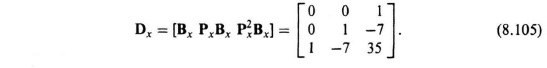
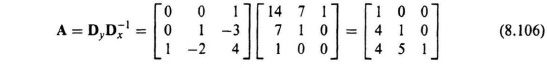
Note that the determinant of D_x is −1 indicating that the determinant is nonsingular, and the phase-variable form is also controllable, as expected. The transformation matrix, defined in Eq (8.85), can be determined from Eqs. (8.97) and (8.105) as follows:

The next step in the procedure is to design the controller (see Figure 8.3) using the phase-variable representation, after which we will transform the design back to the original system by using Eq (8.106). The 4.33 percent overshoot specified can be obtained from a second-order control system having a damping ratio of 0.707 [see Eq. (4.33)]. The settling time of 6 sec can be obtained from a second-order control system having a damping ratio of 0.707 and a ω_n = 0.943 [see Eq. (5.41)]. Therefore, the following second-order control system can meet the design specifications:

Since it was shown in Section 8.2 that zeros of closed-loop systems are zeros of open-loop systems, then we can select the third pole at s = −3 which will also cancel the zero at s = −3. Therefore, the characteristic equation of the desired closed-loop system is

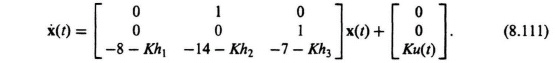
The state and output equations for the phase-variable form with linear-state-variable-feedback can be obtained from Eqs. (8.8), (8.9), and (8.10) as follows:

Eq. (8.109) reduces to the following:

The resulting characteristic equation can be obtained from Eqs. (8.10) and (8.19):

Substituting −(P_x − Kb_xh_x) from Eq (8.111) into Eq (8.112), we obtain the following:

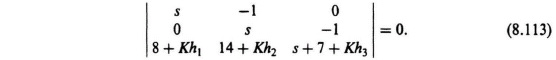
The resulting characteristic equation is given by:

Comparing Eq (8.114) and Eq (8.108), we obtain the following three equations:

Therefore,

We will now transform Kh_x as shown in Eq (8.118) back to the original system using Eq (8.94) and Eq (8.106) as follows:

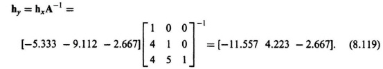
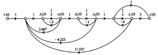
Figure 8.17  Resulting closed-loop control system with linear-state-variable-feedback designed using Ackermann’s Formula.

The resulting closed-loop control system with linear-state-variable-feedback is shown in Figure 8.17.