4.4.  STATE-VARIABLE SIGNAL-FLOW GRAPH OF A SECOND-ORDER SYSTEM

In the previous section, the derivation of the time response of the second-order system was based on the transfer-function derivation. Therefore, an implicit assumption was made that the initial conditions were zero. This section illustrates how the state-variable signal-flow graph method of the underdamped case yields a more versatile and complete solution in the time domain including the response to the initial condition terms.

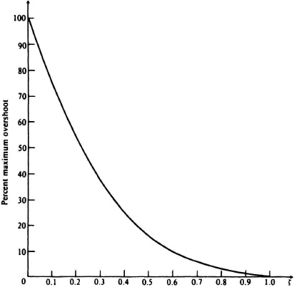
Figure 4.5   Percent maximum overshoot versus damping ratio for a second-order system.

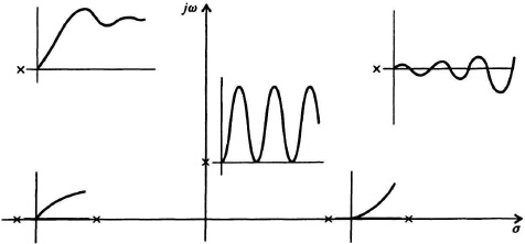
Figure 4.6   Responses of a second-order control system for various root locations in the s-plane (conjugate roots are not shown).

The state-variable signal-flow graph for this system can be derived from Eq. (4.3) as follows:

Dividing through by s², we obtain

Defining

we may rewrite Eq. (4.34) as

From Eq. (4.36) and

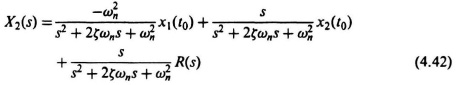
the state-variable signal-flow graph for this system can easily be obtained as illustrated in Figure 4.7. The initial conditions are assumed to occur at t = t₀. Application of Mason’s theorem (Eq. 2.135) to this diagram permits us to write the state equations directly as follows:

where

Simplifying Eqs. (4.38), (4.39), and (4.40), we obtain the following set of equations:

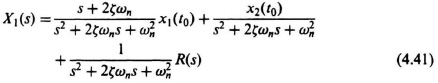
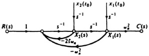
Figure 4.7   State-variable signal-flow graph of a second-order system.

These two equations can be put into the following vector form:

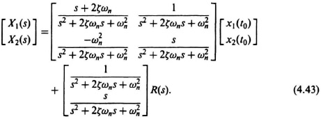
The inverse Laplace transform of Eq. (4.43) is given by the following expression (it is assumed that R(s) = 1/s and that ζ < 1):

where

Notice from this approach that the state transition matrix is readily available.

The corresponding output response of this second-order system having a unit step input is given by the following expression:

Equation (4.45) is a much more complete solution to the classical second-order system than that previously derived in Eq, (4.24), since the initial conditions are now accounted for. Observe from Eq. (4.45) that the solution, when the initial conditions are zero, reduces to that of Eq. (4.24) with α = −₂. The first term in Eq. (4.45) represents the forced response due to the external forcing function, and the last two terms represent the natural or homogeneous solutions due to the initial conditions.