
6.4. MAPPING CONTOURS FROM THE s-PLANE TO THE F(s)-PLANE
Prior to introducing the Nyquist stability criterion which is very useful for determining the degree of stability or instability of feedback control systems, it is important to understand how to map contours from the s-plane to the F(s)-plane where F(s) is some rational function of s. A contour map is defined as a contour in the s-plane which is then mapped or transferred into the F(s)-plane by the definition of the rational function F(s). Because s is the complex variable s = σ + jω and F(s) is a complex function, then we can represent F(s) as F(s) = u + jv. Therfore, the F(s)-plane is also a complex plane having coordinates of u and v.
To illustrate the mapping process from the s-plane to the F(s)-plane, consider the unit-square contour in the s-plane illustrated in Figure 6.5a. We wish to map this unit-square contour from the s-plane to the F(s)-plane where F(s) is a rational function of s and is defined by the following expression:
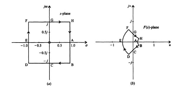
Figure 6.5 (a) Contour in the s-plane to be mapped for F(s) = s/(s + 3). (b) Resulting mapping in the F(s)-plane for F(s) = s/(s + 3) for the contour shown in the s-plane in Figure 6.5(a).
Since we are defining F(s) = u + jv, then
Table 6.1 provides several values of F(s) as s traverses the unit-square contour of the s-plane illustrated in Figure 6.5a. Observe that for each point in the s-plane, there is only one corresponding point in the F(s)-plane. Therefore, the mapping from the s-plane into the F(s)-plane is one-to-one. The resulting contour in the F(s)-plane is illustrated in Figure 6.5b. The points A, B, C, D, E, F, G, and H illustrated in the contour map in the s-plane map into the corresponding points A, B, C, D, E, F, G, and H in the F(s)-plane. We conclude that the unit-square contour of the s-plane maps into a different-shaped cotour in the F(s)-plane as illustrated in Figure 6.5b. We also conclude that a closed contour in the s-plane results in a closed contour in the F(s)-plane.
Another important point to recognize is the direction of the contour. Arrows are shown in Figure 6.5a of the traversal of the unit-square in the s-plane in going from A to B to C to D to E to F to G to H and back to A. A corresponding traversal occurs in the F(s)-plane contour as illustrated in Figure 6.5b. By convention in control systems, the area within a contour to the right of the traversal (as viewed by an observer standing on the contour and facing in the direction of the traversal) is defined as the area enclosed by the contour. Another convention in control systems is to consider a clockwise traversal of the contour to be positive. The direction and number of encirclements of the origin in the F(s)-plane by the closed contour is very significant in the Nyquist diagram which is discussed in the following section where we will correlate the number and direction of encirclements of the origin of the F(s)-plane with the stability of the control system.
It is significant that the path we chose for s in Figure 6.5a did not go through any singular points such as the pole of F(s) at −3 but it did contain the zero of F(s) at the origin. The result was a closed contour in the F(s)-plane which enclosed the origin of the F(s)-plane in the clockwise direction. The number of encirclements of the origin of the F(s)-plane depends on the closed contour in the s-plane. For example, if we have a contour that encloses one pole in the s-plane and the contour encircles the origin in the s-plane in the clockwise direction, then the contour in the F(s)-plane encloses the origin in the F(s)-plane in the counterclockwise direction. This is illustrated in Figure 6.6a and b for the following function:
Table 6.1. Corresponding Values in the s-Plane and F(s)-Plane for Figures 6.5a and b, respectively
| Point | s = σ + jω | F(s) = u + jv |
| A | 1 | 0.25 |
| B | 1 − j | 0.29 − 0.18j |
| C | −j | 0.1 − 0.3j |
| D | −1 −j | −0.2 − 0.6j |
| E | −1 | −0.5 |
| F | −1 + j | −0.2 + 0.6j |
| G | j | 0.1 + 0.3j |
| H | 1 + j | 0.29 + 0.18 |
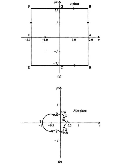
Figure 6.6 (a) Contour in the s-plane to be mapped for F(s) = 1/(s + 1). (b) Resulting mapping in the F(s)-plane for F(s) = 1/(s + 1) for the contour shown in the s-plane in Figure 6.6 (a).
The clockwise contour illustrated follows the path ABCDEFGHA and encloses the pole at s = −1. The corresponding contour in the F(s)-plane, illustrated in Figure 6.6b, shows that the closed contour ABCDEFGHA encircles the origin of the F(s)-plane in the counter-clockwise direction. Table 6.2 tabulates several values of F(s) as s traverses the contour of the s-plane illustrated in Figure 6.6a.
As a third illustration on mapping contours from the s-plane to the F(s)-plane, let us consider the contour ABCDEFGHA traversed in Figure 6.7a which encloses the pole and zero terms for the following function:
The corresponding contour in the F(s)-plane is illustrated in Figure 6.7b. Table 6.3 provides several values of F(s) as s traverses the contour illustrated in Figure 6.7a. Figure 6.7b shows that the resulting contour does not enclose the origin in the F(s)-plane. This clearly illustrates that the encirclement of a pole and a zero in the s-plane does not result in an encirclement of the origin of the F(s)-plane because the zero cancels the effect of the pole. (The clockwise encirclement of a zero alone in the s-plane would result in a clockwise encirclement of the origin in the F(s)-plane, while a clockwise encirclement of a pole alone in the s-plane would result in a counterclockwise encirclement of the origin in the F(s)-plane.)
This analysis illustrates that if there is an encirclement of the origin of the F(s)-plane, its direction depends on whether the contour in the s-plane encloses a pole(s) and/or zero(s). The results derived are now summarized:
Table 6.2. Corresponding Values in the s-Plane and F(s)-Plane for Figures 6.6a and b, respectively
| Point | s = σ + jω | F(s) = u + jv |
| A | 2 | 0.33 |
| B | 2 − 2j | 0.23 + 0.15j |
| C | −2j | 0.2 − 0.4j |
| D | −2 − 2j | −0.2 + 0.4j |
| E | −2 | −1 |
| F | −2 + 2j | −0.2 − 0.4j |
| G | 2j | 0.2 − 0.4j |
| H | 2 + 2j | 0.23 − 0.15j |
Table 6.3. Corresponding Values in the s-Plane and F(s)-Plane for Figures 6.7a and b, respectively
| Point | s = σ + jω | F(s) = u + jv |
| A | 2 | 0.67 |
| B | 2 − 2j | 0.77 − 0.15j |
| C | −2j | 0.8 − 0.4j |
| D | −2 − 2j | 1.2 − 0.4j |
| E | −2 | 2 |
| F | −2 + 2j | 1.2 + 0.4j |
| G | 2j | 0.8 + 0.4j |
| H | 2 + 2j | 0.77 + 0.15j |
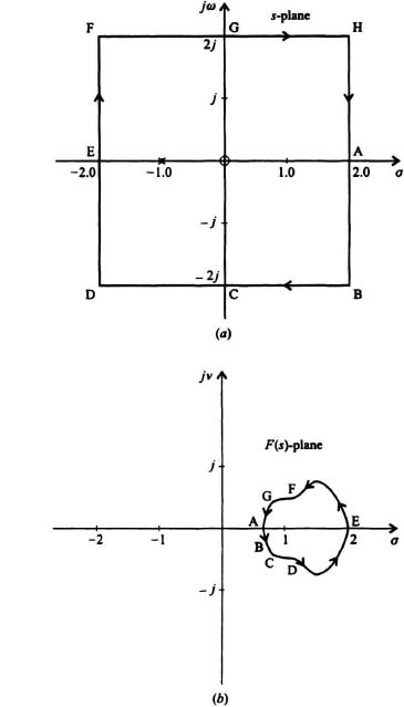
Figure 6.7 (a) Contour in the s-plane to be mapped for F(s) = s(s + 1). (b) Resulting mapping in the F(s)-plane for F(s) = s/(s + 1) for the contour shown in the s-plane in Figure 6.7(a).
1. If a clockwise contour in the s-plane encloses one zero as illustrated in Figure 6.5a, then the origin of the F(s)-plane will have a contour encircling it once in the clockwise direction as illustrated in Figure 6.5b. If there are two (or more) zeros contained within the contour in the s-plane, then the contour in the F(s)-plane will encircle in the clockwise direction the origin two (or more) times.
2. If a clockwise contour in the s-plane encloses one pole as illustrated in Figure 6.6a, then the origin of the F(s)-plane will have a contour encircling it in the counter clockwise direction as illustrated in Figure 6.6b. If there are two (or more) poles contained within the contour in the s-plane, then the contour in the F(s)-plane will encircle in the counterclockwise direction the origin two (or more) times.
3. If a clockwise contour in the s-plane encloses both poles and zeros, then the origin of the F(s)-plane will have a contour encircling it whose net counterclockwise (or clockwise) encirclements will equal the difference of the poles and zeros (zeros and poles) enclosed by the contour in the s-plane. If the number of poles and zeros contained within the contour of the s-plane are equal, as illustrated in Figure 6.7a, then the contour in the F(s)-plane will not encircle the origin as illustrated in Figure 6.7b.
This graphical analysis of mapping from the s-plane to the F(s)-plane is the basis of the Nyquist stability criterion discussed in Section 6.5.