5.5.  TRANSIENT RESPONSE

In addition to stability, sensitivity, and accuracy, we are always concerned with the transient response of a feedback system. Transient response characteristics are defined on the basis of a step input. The response of a second-order system, containing one pure integration, to a unit step is useful for purposes of defining the various transient parameters. Should a problem arise where the system is higher than second order, a reasonably good approximation can be made by assuming that the system is second order if one pair of complex-conjugate roots dominates. This point is amplified during the discussion of the root locus in Chapters 6, 7 and 8. For purposes of illustration, let us consider the second-order system analyzed in Section 4.2. There we had a unity-feedback system whose closed loop transfer function C(s)/R(s) was given by [see Eq. (4.3)]

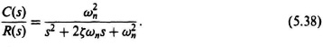
Its response to a unit step input, for the case of ζ < 1, was given by [see Eq. (4.24)]

where

The input and output responses are illustrated in Figure 5.7.

The time for the feedback system to reach its first peak of the overshoot is commonly referred to as the time to peak t_p As was derived in Section 4.2 [see Eq. (4.30)] and is illustrated in Figure 5.7,

or

The time required for the system to damp out all transients is commonly called the settling time t_s. Theoretically, for a second-order system this is infinity. In practice, however, the transient is assumed to be over when the error is reduced below some minimum value. Typically, the minimum level is set at 2% of the final value. The settling time, which is approximately equal to four time constants of the envelope of the damped sinusoidal oscillation, is illustrated in Figure 5.7 and is given by

The rise time t_r is defined as the time required for the response to rise from 10% to 90% of its final value. Figure 5.7 illustrates the rise time for the response shown. Figure 5.8 illustrates the resulting curve obtained relating the variation of ω_nt_r and the damping factor, ζ. Using MATLAB, a third-order fit was made to the curve and the following expression was obtained:

ω_nt_r = 1.589ζ³ − 0.1562ζ² + 0.9247ζ + 1.0141.

Notice that this fit is so close to the actual curve, it is hard to distinguish between these two curves. Solving for t_r we obtain the following:

If a simple expression is desired for approximations, we can obtain the values of t_r over the desirable range of damping factors, from 0.4 to 0.7 (as discussed in Section 4.5), and then determine an average value over this range. The value of ω_nt_r for a damping of 0.4 is 1.4635; the value of ω_nt_r for a damping of 0.7 is 2.1299. Therefore, an average value of rise time over this damping factor range is given by

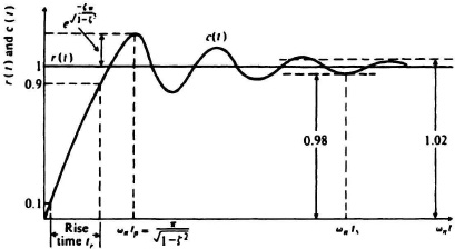
Figure 5.7   Response of a second-order system to a unit step.

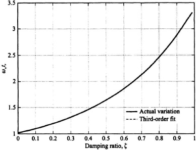
Figure 5.8   Variation of undamped natural frequency times rise time as a function of damping ratio.

This is a reasonable approximation to use for determining the rise time of second-order systems or systems that can be approximated as second-order systems (which is discussed further in Chapter 7).

The rise time is a useful characteristic for underdamped, critically damped, and overdamped systems. The time to peak is useful only for underdamped systems.

As is illustrated in Figure 5.7, a second-order system will have an exponentially decaying sinusoid when the damping factor is between 0 and 1 (this was derived in Section 4.2).

The first overshoot is of particular interest; the ratio of this overshoot’s peak value to the steady-state settling value of the system is expressed as a percentage. The amount of overshoot allowable depends entirely on the particular problem. (see Section 4.5.) Notice that the percentage overshoot of the system illustrated in Figure 5.7 is exp(− [see Eq. (4.33)].

Even though reasonable values for time to peak, rise time, settling time, and the peak overshoot have been chosen, one is not sure whether a good system has been designed. For example, if the rise time is very small, invariably the peak value of the overshoot increases and so does the settling time. On the other hand, if the design is for minimum overshoot, the rise time increases. In order to resolve the conflict that exists between rise time, peak overshoot, and settling time, criteria have been proposed for synthesizing optimum transient performance for linear systems. Most of these criteria consider that the error and/or the time at which the error has occurred during the transient is important [1, 2]. Several of these criteria are presented in the remainder of this chapter.