7.6.  COMPENSATION AND DESIGN USING THE BODE-DIAGRAM METHOD

The techniques necessary to construct and analyze the open-loop frequency response of a feedback control system utilizing the Bode-diagram approach were presented in Section 6.7. This section illustrates how the Bode diagram can be used for designing a feedback-control system in order to meet certain specifications regarding relative stability, transient response, and accuracy. It is important to emphasize that the Bode-diagram approach is used very frequently by the practicing control engineer. Its use is due to the fact that the anticipated theoretical results may be relatively simply checked with actual performance in the laboratory just by opening the feedback loop and obtaining an open-loop frequency response of the system.

Bode’s primary contribution to the control art is summarized in two theorems [7]. We introduce the concepts embodied in these theorems first in a qualitative manner, and then the mathematical statements are given.

A.  Bode’s Theorems

Bode’s first theorem essentially state that the slopes of the asymptotic amplitude–log-frequency curve implies a certain corresponding phase shift. For example, in Section 6.7 it was shown that a slope of 20n dB/decade (or 6n dB/octave) corresponded to a phase shift of 90n° for n = 0, ±1, ±2, …. Furthermore, this theorem states that the slope at crossover (where the attenuation–log-frequency curve crosses the 0-dB line) is weighted more heavily toward determining system stability than a slope further removed from this frequency. This results in a rather complex weighting factor which is a measure of relative importance toward determining system stability.

From what has been presented so far, this theorem is intuitively seen to be valid. Gain crossover frequency is one of the two points that is checked to determine the degree of stability when using the Bode diagram. Specifically, the phase shift is measured at this particular frequency in order to determine the phase margin. A feedback system whose slope at gain crossover is −20 dB/ decade, and whose other slope sections are relatively far away from crossover in accordance with the relative weighting function, implies a phase shift of approximately −90° in the vicinity of crossover and a corresponding phase margin of about 90°. This value of phase margin certainly implies a stable system. A system, however, whose slope at crossover is −40 dB/decade, and whose other slope sections are relatively far away from crossover in accordance with the relative weighting function, implies a phase shift of approximately −180° and a corresponding phase margin of about 0°. This value of phase margin implies a system which is on the verge of being unstable and would probably be so when actually tested. Steeper slopes would indicate negative phase margins and definitely unstable systems. Therefore, one strives to maintain the slope of the amplitude–log-frequency curve in the area of gain crossover at a slope of −20 dB/decade. Notice that the system, illustrated in Figure 6.33, has slopes of −60 dB/decade that are relatively far from the gain crossover frequency. Therefore, this system has a fairly respectable phase margin of 56.74° by maintaining the 20 dB/decade slope for about an octave below, and about 2 octaves above crossover.

Bode’s second theorem essentially states that the amplitude and phase characteristics of linear, minimum-phase-shift systems are uniquely related. When we specify the slope of the amplitude–log-frequency curve over a certain frequency interval, we have also specified the corresponding phase-shift characteristics over that frequency interval. Conversely, if we specify the phase shift over a certain frequency interval, we have also specified the corresponding amplitude–log-frequency characteristic over that frequency interval. The theorem emphasizes the fact that we can specify the amplitude–log-frequency characteristic over a certain interval of frequencies together with the phase-shift–log-frequency characteristics over the remaining frequencies. It should be emphasized that these conclusions apply only if the transfer function is minimum phase.

The second theorem may appear quite trivial at first glance. Its implications however, are quite important. We will make further use of this this theorem when designing feedback control systems using the Bode-diagram approach.

The formal mathematical statement of Bode’s first theorem is given by the following expression:

where (ω_d) is the phase shift of the system in radians at the desired (e.g., crossover) frequency ω_d, G represents the gain in nepers (1 neper = 1n|e|), n = 1n(ω/ω_d),|dG/dn| represents the slope of the amplitude–log-frequency curve in nepers per unit change of n (1 neper/unit change of n is equivalent to 20 dB/decade), |dG/dn|_d is the slope of the amplitude–log-frequency curve at the desired (crossover) frequency ω_d, and 1n coth|n/2| is the weighting function which is plotted in Figure 7.20. The first term of Eq. (7.58) represents the phase shift contributed by the slope of the amplitude–log-frequency curve at the reference frequency ω_d. For example, it yields a phase shift of 90° for every neper per unit of n (20 dB/decade). The second term of Eq. (7.58) is proportional to the integral of the product of the weighting function and the difference in slope of the amplitude–log-frequency curve at a frequency ω as compared to its value at the reference frequency, ω_d. Attention is drawn to the fact that it is the weighting function that determines the phase-shift contribution at ω_d due to the amplitude–log-frequency curve which exists at some frequency ω. Because the second term of Eq. (7.58) is zero for large values of n and where n = 0, the value of the integral will be relatively small compared with the first term if the slope of dG/dn is constant over a relatively wide range of frequencies above ω_d. Therefore, under these conditions, the phase shift would be determined primarily by the first term of Eq. (7.58). Following this line of reasoning, the slope of the amplitude–log-frequency curve should be less than −2 nepers per unit of n (−40 dB/decade) over a relatively wide range of frequencies at crossover in order to ensure stability.

The formal mathematical statement of Bode’s second theorem is given by the following expression:

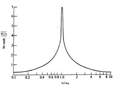
Figure 7.20   Plot of the weighting function used in Bode’s first theorem.

where ω_s represents the frequency in radians per second below which the amplitude–log-frequency characteristics is specified and above which the phase characteristic is specified. This theorem emphasizes the interdependence of amplitude and phase shift over the entire range of positive frequencies. In addition, notice that although it is possible to specify amplitude or phase in one range of frequencies, and the other quantity in the remaining frequencies, these quantitites reflect their presence back into the other range of frequencies. Therefore the integration with respect to frequency is performed over the entire range of positive frequencies.

The design of several systems using the Bode-diagram approach is considered next. We shall illustrate a method that determines steady-state accuracy from the Bode diagram as well as meeting relative stability requirements.

B.  Example of Phase-Lead and Phase-Lag Network Compensation, and Rate-Feedback Compensation

Let us first consider the third-order system illustrated in Figure 7.21a. Its open-loop transfer function G₀(s) is given by

The Bode diagram for the uncompensated system [G_c(s) = 1] is illustrated in Figure 7.22. It shows a gain crossover frequency of 33.78 rad/sec, a phase margin of −3.402°, and a gain margin of −1.1422 dB. The frequency where the phase shift equals −180° (phase crossover frequency) is 31.7 rad/sec. This Bode diagram was obtained using MATLAB, and is contained in the M-file that is part of my Modern Control System Theory and Design (MCSTD) Toolbox can be retrieved free from The MathWorks, Inc. anonymous FTP server at ftp://ftp.mathworks.com/pub/books/shinners.

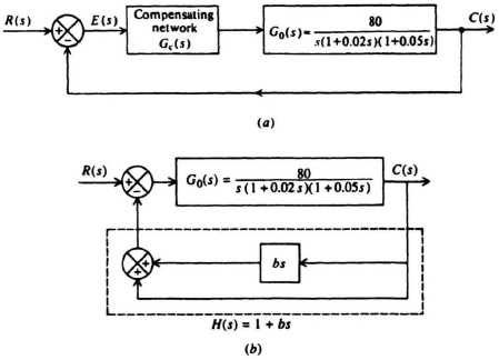
Figure 7.21   A third-order system which is to be compensated using (a) cascade compensation (phase-lag and phase-lead) and (b) rate-feedback compensation.

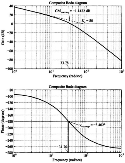
Figure 7.22   Third-order system where the uncompensated transfer function is

These results indicate that the uncompensated system is unstable. Let us next attempt to compensate this system with a phase-lag network, a phase-lead network, and the use of rate feedback in parallel with position feedback (which produces a pure zero factor). The specifications for this sytem require a minimum phase margin of 20° and a minimum gain margin of 10 dB. In addition, it is assumed that a sinusoidal disturbance at 1 rad/sec is present, and a gain of at least 35 dB is required at this frequency to nullify its effect.

1. Phase-Lag Network Compensation Let us first consider the phase-lag-network compensation case in Figure 7.21. Applying Bode’s theorems in order to achieve the specified phase and gain margins, we would expect that the −20 dB decade slope in the vicinity of the new crossover frequency should not extend over too wide a range of frequencies because the relative stability that is desired is rather moderate. The phase-lag network is of the form.

where αT > T. In Section 7.2 we studied the characteristics of the phase-lag network. In particular, Figure 7.9 illustrated the Bode diagram of a general phase-lag network. Notice that this type of network is of such a nature that it attenuated all high-frequency components above ω = 1/T by a factor of 1/α. From the Bode-diagram viewpoint, this attenuating characteristic can be used for stabilization purposes by reshaping the uncompensated amplitude characteristics, so that the initial −20 dB/decade is made to cross over the 0-dB line rather than the −40-dB/decade segment. In other words, one would attempt to stabilize this system with a phase-lag network by placing the frequencies 1/αT and 1/T in the range of frequencies below about 10 rad/sec. It would be desirable that the −20-dB/decade segment start at least around 10 rad/sec cross over the 0-dB line before 20 rad/sec where the amplitude–log-frequency characteristic changes to a slope of −40 dB/decade. In addition, we would not want 1/αT to occur at less than 1 rad/sec, because an open-loop gain of 35 dB has been specified at ω = 1 rad/sec. The final phase of the solution is by means of iteration. However, the procedure converges quite rapidly. Usually, two or three iterations should prove sufficient. For the requirements specified, a phase-lag network given by

results in a gain crossover frequency of 11.371 rad/sec, a phase margin of 20.978° and a gain margin of 10.988 dB as shown in Figure 7.23. The frequency where the phase is −180° (phase crossover frequency) occurs at 24.22 rad/sec.

2. Phase-Lead Network Compensation. Let us next consider the phase-lead-network compensation case. The lead network has the form

where αT > T. In Section 7.2 we studied the characteristics of the phase-lead network. We assume that any low-frequency attenuation, which is due to the value of 1/α, is made up for by increasing the gain of the feedback control system by a like amount. The Bode diagram of a general phase-lead network was shown in Figure 7.11. From the Bode-diagram viewpoint, this type of characteristic can be used for stabilization purposes by reshaping the uncompensated amplitude characteristics so that a −40-dB/decade slope is made to cross over the 0-dB line along a synthesized −20-dB/decade slope rather than the −40-dB/decade segment. The range of frequencies where one can place the frequencies 1/αT and 1/T is quite limited in this particular problem. The value of 1/αT can be placed between 20 and 33.78 rad/sec. The closer it is to 20 rad/sec, the greater its stabilizing effect. The further away the break 1/T is from 33.78 rad/sec, the greater will be the stabilizing effect of the phase-lead network. It can be seen that this particular solution does not modify the open-loop characteristics in the vicinity of 1 rad/sec and the accuracy specification of 35 dB at 1 rad/sec will easily be achieved.

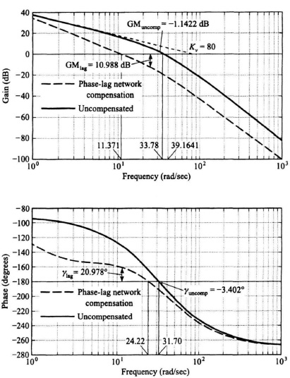
Figure 7.23   Compensation of a third-order system with a phase-lag network of G_c(s) = (1 + 0.143s)/(1 + s) where the uncompensated transfer function is

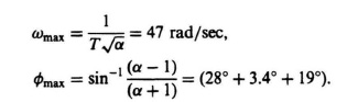
We can obtain the pole and zero terms in Eq. (7.63) using a first-cut design procedure by using Eqs. (7.7) and (7.8) for the phase-lead network and the following reasoning. Equation (7.7) states the frequency where the maximum phase lead occurs, and Eq. (7.8) states the maximum value of the phase lead. In view of the analysis of the previous paragraph, it seems reasonable to place the frequency where maximum phase lead occurs around 47 rad/sec, and to make _max equal to the phase margin desired (a conservative choice of 28° will be selected) plus the magnitude of the phase margin obtained of the uncompensated system (because it is negative) at the gain crossover frequency of 33.78 rad/sec (3.402°) plus the additional phase shift that the composite phase shift curve incurs in going from the uncompensated crossover frequency of 33.78 rad/sec to ω_max of 47 rad/sec (about 19°) as follows:

Solving these two equations simultaneously, we obtain the phase-lead network

Because this solution has “blinders” on and does not consider the proximity of other poles and zeros, it usually has to be fine-tuned. Therefore, the following phase-lead network was selected and is illustrated in Figure 7.24:

It results in a phase margin of 28.431° and a gain margin of 10.655 dB. This meets the specification requirements. Notice that the resulting phase-lead network has a low-frequency attenuation of 0.005/0.04 which must be made up by increasing the gain by a factor of 0.04/0.005 = 8. Its gain crossover frequency is 47.27 rad/sec, and the phase crossover frequency occurs at 94.06 rad/sec.

If we have a choice of using the phase-lag or phase-lead network, the phase-lag network solution would be preferable because it meets the required specifications with a narrower bandwidth than the phase-lead network case (ω_c = 11.371 rad/sec for the former; ω_c= 47.27 rad/sec for the latter). A feedback control system having a narrower bandwidth will reject a greater amount of noise than one having a wider bandwidth, as well as requiring less power and cost. In addition, the phase-lead network has the disadvantage of requiring a greater amount of amplification within the control system than the phase-lag network. These and other considerations are discussed further in Section 7.10, where tradeoffs of using different kinds of cascade networks and minor-loop feedback compensation methods are compared.

3. Rate Feedback in Parallel with Position Feedback Compensation. Finally, we wish to compensate the system using rate-feedback compensation in parallel with position feedback as shown in Figure 7.21b. The addition of rate feedback provides an H(s) term of

H(s) = (1 + bs)

which represents a pure zero term that provides a phase lead of

tan⁻¹ bω = _max.

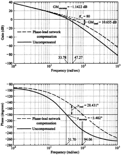
Figure 7.24   Compensation of a third-order system with a phase-lead network G_c(s) = (1 + 0.04s)/(1 + 0.005s) where the uncompensated transfer function is

Remember that a pure zero term is an ideal compensator. Using a similar procedure as for the design of the phase-lead network, let us assume that we desire an approximate 50° phase lead at a frequency of 50 rad/sec. Therefore,

b(50) = tan 50°
       b = 0.0238.

The use of rate-feedback compensation is illustrated in Figure 7.25 and indicates a phase margin of 31.9728° at the gain crossover frequency of 39.1641 rad/sec. Its gain margin is infinity, because the phase never is −180° except at ω = infinity.

Figure 7.26 illustrates the Bode diagram of the uncompensated system, and the Bode diagram of the compensated systems with a phase-lag network, phase-lead network, and with rate feedback in parallel with position feedback all superimposed on one Bode diagram.

Figure 7.25   Compensation of third-order system with rate feedback (b = 0.0238) in parallel with position feedback where the uncompensated transfer function is

C.  Obtaining Steady-State Error Coefficients from the Bode Diagram

The steady-state error coefficients can be determined from the Bode diagram. The definition and importance of these error coefficients have been discussed in Section 5.4. For a system having one pure integration, the velocity constant K_v can be obtained by extending the initial −20-dB/decade slope until it intersects the 0-dB line. The frequency at which it intersects this line is equal to the velocity constant. We recall from our discussion in Section 5.4 that K_v was obtained by letting s approach zero when utilizing the final-value theorem [see Eq. (5.18)]. Therefore, the pole and/or zero terms having the forms (1 + Ts) or [(Ts)² + 2ζTs + 1] all approach unity. This permits one to obtain K_v directly by considering only the initial slope of the Bode diagram. For the Bode diagram shown in Figures 7.22–7.26, the value K_v obtained graphically is 80. As a check, using the definition given by Eq. (5.18), we obtain

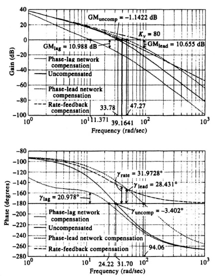
Figure 7.26   Compensation of a third-order system where the uncompensated transfer function is

Because

then,

It is also interesting to note that the velocity constant is the same for the uncompensated and compensated systems.

For a system which has a double pole at the origin, the acceleration constant K_a can be obtained in a similar manner. The initial −40-dB/decade slope is extended until it intersects the 0-dB line. The square of the frequency at which it intersects this line is equal to the acceleration constant.

D.  Example of Compensating a System Containing a Disturbance Input

The next system we consider is illustrated in Figure 7.27. This consists of a third-order system which has an unwanted external input U(s). The open-loop transfer function for the uncompensated system, G₀(s), is given by

It is desired that the steady-state error resulting from an unwanted, external step input signal at U(s), should not exceed 0.1 unit. The compensation device, G_c(s), is to contain amplification which will meet this accuracy requirement together with a phase-lead or phase-lag network which will provide a minimum phase margin of 20° and a minimum gain margin of 6 dB.

The value of gain K required for G_c(s) will be computed first. For this calculation, U(s) is assumed to be the input and E(s) is assumed to be the output. The transfer function between these two points is given by

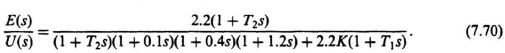
Setting U(s) = 1/s, we obtain the expression for the Laplace transform of the error, E(s), as

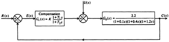
Figure 7.27   A third-order system having an unwanted external input.

The required value of K can be obtained by applying the final-value theorem to E(s) and setting the result equal to 0.1 unit. We find

Let us next determine the compensating network required to achieve a phase margin of 20° and a gain margin of 6 dB. The transfer function of the uncompensated system, with K = 9.55, is given by

Its Bode diagram which is drawn in Figure 7.28, indicates a phase margin of 0.7167° (gain crossover frequency is 5.8668 rad/sec) and a gain margin of 0.267 dB (phase crossover frequency is 5.9522 rad/sec). We wish to increase the phase margin by about 20°. This Bode diagram was obtained using MATLAB and is contained in the M-file that is part of my MCSTD Toolbox and can be retrieved free from The MathWorks, Inc. anonymous FTP server at ftp://ftp.mathworks.com/pub/books/shinners.

Figure 7.28   Compensation of a third-order system where

Solid line = uncompensated; dashed line = compensated

As in the previous problem analyzed, in this section, we will estimate the values of ω_max and _max for Eqs. (7.7) and (7.8), respectively, to obtain a first-cut design. We must be careful when using this approach, because we actually want to have this phase shift at the gain crossover frequency in order to achieve the desired phase margin. However, specifying α, T, and ω_max does not ensure that _max will be at the gain crossover frequency. After obtaining this first-cut design, we then fine-tune the results to obtain the specification requirements as in the previous example. For this design and an anlysis of the Bode diagram of the uncompensated system shown in Figure 7.28 a value of ω_max = 8 rad/sec was selected. The value of _max selected was a conservative value of 34° which includes the difference between the minimum phase margin desired (20°) and the actual phase margin of the uncompensated system (0.7167°) plus the difference in phase shift between the gain crossover frequency of the uncompensated system (5.8668 rad/sec) and 8 rad/sec plus an extra margin to be conservative. The resulting two equations to be solved simultaneously were

The result is a phase-lead network whose transfer function is

The first-cut design was adjusted a little to better fit the overall Bode diagram and the final phase-lead network selected is as follows:

This network causes a gain crossover frequency of 6.9778 rad/sec where the phase margin is 21.71°, and a gain margin of 7.955 dB (the phase crossover frequency is at 11.5247 rad/sec). This satisfies the specification. Remember that this network will require an increase in the amplifier gain by 3.34 to make up for the attentuation of 0.05/0.167 = 0.2994 that it provides.

E.  Example for Compensating a Two-Loop System Using Rate Feedback in Cascade with a Filter

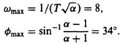
The concluding problem we consider using the Bode-diagram approach consists of designing the feedback control system illustrated in Figure 7.29a. For this particular system, we desire that the steady-state error resulting from a velocity input of 110 rad/sec be equal to 0.25 rad. The uncompensated open-loop transfer function G₀(s) is given by

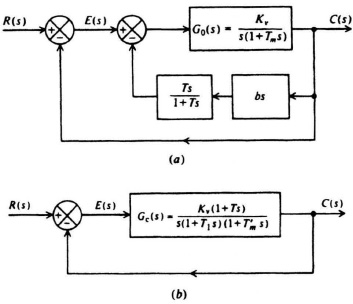
Figure 7.29   (a) Use of rate feedback in cascade with a high-pass filter in order to compensate a feedback control system. (b) Equivalent block diagram for the system shown in (a).

where K_v = velocity constant and T_m = motor time constant = 0.025 sec. This transfer function consists of an amplifier, positioning motor, gear train, and load. In order to achieve the required accuracy, K_v must equal

We want a phase margin of approximately 55° for this system. This will be achieved by means of minor-loop rate-feedback compensation which is cascaded with a simple RC high-pass filter (phase-lead network) in order not to increase the steady-state response error for velocity inputs. This was discussed in Section 7.3 (see Figure 7.15).

The open-loop frequency response we must plot on the Bode diagram is that obtained with the minor-rate loop closed and the outer position loop opened. Therefore, we are interested in obtaining the equivalent transfer function between E(s) and C(s). This is easily found to be

Expanding the denominator of Eq. (7.77), we obtain the expression

This expression can be put into the form

by defining the time constants and T₁ as

and

Therefore, we may redraw Figure 7.29a as shown in Figure 7.29b. For any set of values for T_m, T, K_v, and b, we can derive and T₁ by solving the simultaneous equations (7.80) and (7.81). Another approach is to choose T and T₁ from the Bode diagram which meets the specified phase margin and solve for the required rate-feedback constant b.

The procedure we follow when compensating this system is to draw the Bode diagram for the uncompensated system in accordance with Eq. (7.75) and then fit the characteristics of the compensated system in accordance with

until a phase margin of 55° is achieved. The compensated characteristic will then determine T and T₁, from which and the rate-feedback constant b can be determined. Figure 7.30 illustrates the Bode diagram of the uncompensated and compensated systems. The phase margin of the uncompensated system is 17.1°. Values of

and

result in a phase margin of 55.36°. From Eq. (7.81), the corresponding value of rate-feedback constant b is 0.0186. Figure 7.30 was obtained using MATLAB and is contained in the M-file that is part of my MCSTD Toolbox.

The type of compensation just illustrated is used quite frequently in practice. In order to really understand what is actually happening, it is important to examine the Bode diagram of Figure 7.30 closely. The net effect of the minor-loop rate feedback has been to move the equivalent motor break frequency from 1/T_m to 1/ by the ratio given in Eq. (7.80). This technique is used quite frequently to compensate power servos. The net effect of the phase-lead network, in the minor-loop feedback path, is to appear as a phase lag, for the equivalent open-loop characteristics of Figure 7.29b. This can be easily understood because we effectively see the reciprocal of the feedback element when looking into a closed-loop system which has an open-loop gain much greater than unity [see Eq. (2.122)]. This is a very important fact that can be utilized to approximate the Bode diagram in preliminary designs. This point is now expanded upon in the following section.

Figure 7.30   Compensation of the system shown in Figure 7.29b.

The complete case study for the design of an angular control system for a robot’s joint is presented in Section 7.4 of Chapter 7 of the accompanying volume. In this problem, the Bode diagram is used for analyzing and designing the control system.