
3.4. TRANSFER-FUNCTION AND STATE-VARIABLE REPRESENTATION OF TYPICAL ELECTROMECHANICAL CONTROL-SYSTEM DEVICES
This section illustrates the procedure used for deriving the transfer function and state-variable representation for commonly used devices from their basic differential equations. Examples of control systems which use electromechanical components are in robots, positioning systems such as tracking radars, guidance control systems, printer controls for computer tape and disk drive systems, and ship and aircraft control systems. An illustration of a control system which uses electromechanical components is illustrated in Figure 3.8 which represents the Operational Flight Trainer to simulate the operation of the MV-22A tilt-rotor, twin engine, vertical short takeoff and landing aircraft.
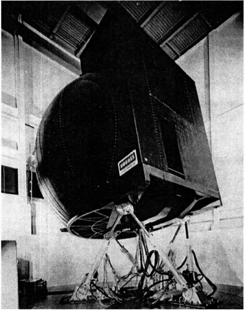
Figure 3.8 The Hughes Operational Flight Trainer simulates the MV-22A tilt-rotor. twin engine, vertical short takeoff and landing aircraft designed for assault support, troop lilt, medical evacuation, and combat search and rescue. This simulator provides training for normal and emergency procedures, visual and instrument flight, and aerial refueling. Software-controlled hydraulic actuators provide six-degree-of-freedom motion to simulate rotary wings, fixed wings, and transition motion. A seat vibrator system simulates aerodynamic and proprotor vibration. (Courtesy of Hughes Training, Inc./Arlington, TX).
We specifically analyze a dc generator, an armature-controlled dc servomotor, a Ward-Leonard system, a field-controlled dc servomotor, and a two-phase ac induction servomotor. The analysis is limited to the linear operating range of these devices.
A. dc Generator
A dc generator [4, 5] is commonly used in control systems for power amplification. The armature, which is driven at a constant speed n, is capable of producing a relatively large controllable current ia(t) as the field current if(t) is varied.
The exact value of ia(t) is dependent on the load circuit impedance ZL. A schematic diagram of the configuration is shown in Figure 3.9. The symbols Rf, Lf, Rg, and Lg represent the resistive and inductive components of the field and armature circuits, respectively.
The voltage induced in the armature, eg(t), is a function of the speed of rotation n(t) and the flux developed by the field ![]() (t). It can be expressed as
(t). It can be expressed as
The flux depends on the field current and the characteristics of the iron used in the field. This is a linear relationship up to a certain saturation point and can be expressed as
By substituting Eq. (3.47) into Eq. (3.46) and assuming that the armature rotation speed is constant, the relation between the induced armature voltage eg(t) and the field current if(t) can be expressed as
where Kg = K1K2n = generator constant having units of V/A. The equation relating the field voltage ef(t) and field current if(t) is
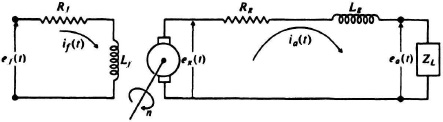
Figure 3.9 dc generator schematic diagram.
The field current can be eliminated between Eqs. (3.48) and (3.49) and an expression relating ef(t) and the induced armature voltage eg(t) can be obtained:
By transforming, there results
The transfer function of this device, defined as the ratio of the output Eg(s) to the input Ef(s), is given by
and its simple block diagram is shown in Figure 3.10.
If it is desired to obtain the transfer function Ea(s)/Ef(s), we must first determine the nature of the actual load connected to the armature. For example, assume that the load impedance is ZL(s). Then the transfer function Ea(s)/Eg(s) becomes
and the overall transfer function of the dc generator, Ea(s)/Ef(s), is
B. Armature-Controlled dc Servomotor
Armature-controlled dc servomotors [6] are quite commonly used in control systems. As a matter of fact, a dc generator driving an armature-controlled dc servomotor is known as the Ward-Leonard system. We will study this configuration next drawing on the relations derived for both the dc generator and armature-controlled dc servomotor.
A schematic diagram of the armature-controlled d servomotor is shown in Figure 3.11a. The symbols Rm and Lm represent the resistive and inductive components of the armature circuit. The field excitation is constant, being supplied from a dc source. The motor is shown driving a load having an inertia J and damping B.

Figure 3.10 Block diagram of a dc generator.
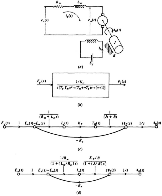
Figure 3.11 (a) Armature-controlled dc servomotor schematic diagram. (b) Block diagram of an armature-controlled dc motor. (c) Signal-flow graph representation for the armature-controlled dc servomotor. (d) Modification of the signal-flow graph to a more compact form.
As the armature rotates, it develops an induced voltage em(t) which is in a direction opposite to ea(t). The induced voltage is proportional to the speed of rotation n(t) and the flux created by the field current. Because we are assuming that the field current is held constant, the flux must be constant. Therefore, the induced armature voltage is only dependent on the speed of rotation and can be expressed as
where Ke = voltage constant of the motor having units of V/(rad/sec). The voltage equation of the armature circuit is
Substituting Eq. (3.55) into Eq. (3.56) and taking the Laplace transform, we obtain
The developed torque of the motor, TD(t), is a function of the ftux developed by the field current, the armature current, and the length and number of the conductors. Because we are assuming that the field current is held constant, the developed torque TD(t) can be expressed as
where KT = torque constant of the motor. The units of KT in the International System are newton meter/ampere, and in the English system are lb ft/ampere.
The developed torque drives the mechanical load and the torque equation is
Substituting Eq. (3.58) into Eq. (3.59) and taking the Laplace transform, we obtain
The overall system transfer function θ0(s)/Ea(s) obtained by eliminating Ia(s) between Eqs. (3.57) and (3.60) is
Equation (3.61) can be defined in terms of an armature time constant Ta, a motor time constant Tm, and a damping factory γ, as follows:
where
The simple block diagram of this system is illustrated in Figure 3.11b.
The state-variable model is derived directly for the armature-controlled dc servomotor from the original set of defining scalar equations, (3.55), (3.56), (3.58), and (3.59). Defining the state variables as
the resulting state equations are given by
In phase-variable canonical form, these equations become
where

It is usually quite interesting and revealing to study the signal-flow graph for such a device, especially for purposes of analog computer simulation. The governing equations from which the signal-flow graph can be drawn for the armature-controlled dc servomotor are given by
The signal-flow graph is illustrated in Figure 3.11c. It clearly illustrates the inherent feedback (back electromotive force) of this device. This property is sometimes used to stabilize a feedback control system (see Problem 3.8). It is left as an exercise to the reader to prove that the transfer function of this system, as derived from the signal-flow graph, agrees with Eqs. (3.62) and (3.63) and that the state equations derived from the state-variable diagram agree with Eqs. (3.70) and (3.71) (see Problem 3.28). For the case of the armature-controlled dc servomotor, the signal-flow graph of Figure 3.11c is modified to a more compact form in Figure 3.11d.
C. The Ward-Leonard System
A configuration having a dc generator driving an armature-controlled dc motor is known as a Ward-Leonard system [7, 8]. The dc generator acts as a rotating power amplifier that supplies the power which, in turn, drives the servomotor. Variations of the conventional Ward-Leonard system are known as the Amplidyne, the Metadyne, the Rotorol, and the Regulex. The reader is referred to more authoritative books on dc machinery [7, 8] for a description of these devices.
A schematic diagram of the basic Ward-Leonard system is shown in Figure 3.12. The notations used are the same as those of Figures 3.9 and 3.11. Many sophisticated variations of this basic configuration, using compensating windings, exist [8].
To enable us to combine the transfer-function relationships derived previously for the dc generator and armature-controlled dc motor, we assume that the generator voltage eg(t) is applied to the armature of the motor. Therefore, we are interested in applying the generator Equation (3.52) rather than (3.54). In order to apply the motor transfer function (3.62), we must first combine the resistive and inductive components of the generator’s and motor’s armatures. It is assumed that Rg is much smaller than Rm, and Lg is much smaller than Lm. This will result in a set of new, modified motor constants as follows:

Figure 3.12 Ward-Leonard system schematic diagram.
Therefore, Eq. (3.62) may be written as follows in this case:
It is now relatively simple to obtain the transfer-function representation of the configuration shown in Figure 3.12. Defining ef(t) as the input and θ0(t) as the output of the system, we need merely to combine the transfer functions given by Eqs. (3.52) and (3.77). Therefore, the system transfer function is given by
and its simple block diagram is illustrated in Figure 3.13.
D. Field-Controlled dc Servomotor
A dc servomotor [9] can also be controlled by varying the field current and maintaining a constant armature current. The schematic diagram of such a configuration, known as the field-controlled dc servomotor, is shown in Figure 3.14. The notations are the same as those of Figure 3.11.
The developed torque of the motor, TD(t), is a function of the flux developed by the armature current, the field current, and the length of the conductors. Because we are assuming that the armature current is held constant, the developed torque TD(t) can be expressed as
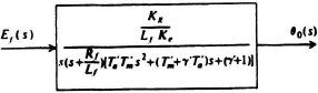
Figure 3.13 Block diagram of the Ward-Leonard system.
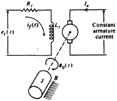
Figure 3.14 Field-controlled dc servomotor schematic diagram.
where KT = torque constant of the motor having units of lb ft/A. The developed torque is used to drive the mechanical load with inertia J and damping B. The torque equation is
Substituting Eq. (3.79) into Eq. (3.80), we obtain a differential equation relating the field current and the output shaft position:
An expression for the value of the field current if(t) can be obtained from the voltage equation of the field circuit:
Substituting Eq. (3.81) into Eq. (3.82) and taking the Laplace transform, we obtain
The transfer function of the device, defined as the output θ0(s) divided by the input Ef(s), is given by
where

and its simple block diagram is illustrated in Figure 3.15a.
The governing equations from which the signal-flow graph can be drawn for the field-controlled dc servomotor are given by

Figure 3.15 (a) Block diagram of a field-controlled dc servomotor. (b) Signal-flow graph representation for the field-controlled dc servomotor.
The simple signal-flow graph of this device is illustrated in Figure 3.15b.
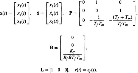
The state-variable equations of the field-controlled dc servomotor can be obtained either by starting from the defining scalar equations, (3.81) and (3.82), or by utilizing the resultant transfer function derived in Eq. (3.84). The first method is usually preferable. However, because the first method was utilized in the case of the armature-controlled dc servomotor, the second method is utilized here for the field-controlled dc servomotor to permit comparison of the two approaches.
Equation (3.84) can be written in differential-equation form as follows:
This third-order differential equation can be written as three first-order differential equations by defining
The resulting state equations are given by
In phase-variable canonical form, these equations become
where
Notice that the resultant vector equation has eliminated the field current. This is a measurable state and it is preferable to retain it in the state-variable model. If the state-variable representation had proceeded from the defining scalar equations, (3.81) and (3.82), then the field current would have been retained—just as the armature current was retained as a state in the case of the armature-controlled dc servo-motor (see Eq. (3.66)].
E. Two-Phase ac Servomotor
The two-phase ac servomotor [10–12] is probably the most commonly used type of servomotor. Its popularity stems from the fact that many error-sensing devices are carrier-frequency (ac) devices. By using two-phase ac servomotors, demodulation need not be performed and ac amplification can be used throughout the electrical portion of the system.
The ac servomotor is a two-phase induction motor having its two stator coils separated by 90 electrical degrees with a high-resistance rotor. A control signal is applied to one phase (the control winding) while the other phase (the reference winding) is supplied with a fixed signal that is phase-shifted by 90° relative to the control signal. The motor is used primarily for relatively low-power applications. A schematic diagram of an ac servomotor driving a load of inertia J and damping B is shown in Figure 3.16. The reference field voltage is denoted as er(t) and the control field voltage is denoted as ec(t). The developed torque of this motor is proportional to er(t), ec(t), and the sine of the angle between er(t) and ec(t). In practice, the reference winding voltage is kept constant at its rated value, the angle between the reference winding and control winding is kept close to 90° by means of a large capacitor placed in series with the reference winding, and the input to the control winding is varied for control purposes.
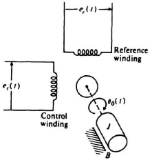
Figure 3.16 Two-phase ac servomotor schematic diagram.
As the control voltage is varied, the torque TD and speed n(t) vary. A set of torque-speed curves for various values of control voltage are shown in Figure 3.17. Notice that these curves show a very large torque for zero speed which is desirable in developing a very rapid acceleration.
Unfortunately, the torque-speed curves are not straight lines. Therefore, we cannot write a linear differential equation to represent them. However, by linearizing these characteristics, reasonable accuracy can be achieved.* Because the developed torque TD is a function of the speed n(t) and the control voltage ec(t), we use a Taylor-series expansion of the nonlinear functin TD(n, ec) to get an approximate linear function:
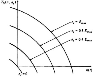
Figure 3.17 Two-phase ac servomotor torque-speed characteristics.
![]()
and substituting n(t) = dθ0(t)/dt, we can rewrite Eq. (3.97) as
The developed torque is used to drive the mechanical load and the torque equation is
Substituting Eq. (3.99) into Eq. (3.98) and taking the Laplace transform, we obtain
The transfer function of the device, defined as the output θ0(s) divided by the input Ec(s), is given by
where
and its simple block diagram is illustrated in Figure 3.18. Although the torque-speed characteristics are nonlinear, as illustrated in Figure 3.17, the value of Kn is usually obtained graphically by drawing a straight line through the two end points. The accuracy of this approach, compared with drawing a line tangent to the curve at various other points, is analyzed further in Chapter 10, Section 10.6 (see Problem 10.1).
In practice, B is usually very small compared to Kn and can be assumed to be negligible.
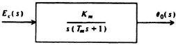
Figure 3.18 Block diagram of a two-phase ac servomotor.
A very important characteristic of the two-phase ac servomotor is the torque-to-inertia ratio which provides a measure of the maximum acceleration that the device can achieve. It is defined as the ratio of the maximum torque at standstill (for the specified control field voltage, ec(t)) to the rotor moment of inertia. The larger the ratio, then the better is the acceleration characteristic of the two-phase ac servomotor.
Equation (3.101) can be written in differential-equation form as follows:
This second-order differential equation can be written as two first-order differential equations by defining
The resulting state equations are given by
In phase-variable canonical form, these equations become
where

It is left as an exercise to the reader to prove that the state equations derived from the state-variable diagram agree with Eqs. (3.107) and (3.108) (see Problem 3.30).
F. Servomotors with Gear Reducers
The two-phase ac servomotor is inherently a high-speed, low-torque device. In control-system practice, however, what is usually needed is a low-speed, high-torque device. Therefore, a gear reduction is usually required between the high-speed, low-torque servomotor and the load to obtain speed reduction and torque magnification.
In order to analyze the modifications necessary to the transfer function derived in Eq. (3.101), let us consider the configuration illustrated in Figure 3.19. The subscripts m and l are used to denote motor and load shafts, respectively. It is assumed initially that the inertias of the gears are negligible, the efficiency of transmission is perfect, and there is only one gear mesh between the load and the motor. It is also assumed that a servomotor and gear train have been selected which will provide the required torque to obtain the desired acceleration, and to drive the load at the maximum required speed. Basically what is desired is a set of relationships to include the effect of the gear reduction and the load inertia.

Figure 3.19 Servomotor geared to load.
There are basically two approaches to the problem. In one method, the parameters Knm, Kem, and Jm are reflected to the output shaft, θl. Another manner of solving the problem is to reflect the load inertia to the motor shaft. Both methods will be illustrated here, and it will be shown that they are equivalent.
Let us first consider the reflection of the paramters Knm, Kem, and Jm to the output shaft θl. Knm is the ratio of motor torque to motor speed and the value of Knm is given by
Because the driving torque at the load is multiplied by the gear-reduction factor N, and the motor speed is reduced by this factor at the load shaft, the following relationship is obtained:
where Knl denotes Kn referred to the load shaft.
The parameter Kem is the ratio of motor torque to control voltage. Because the driving torque of the load is multiplied by the gear reduction factor N, and the control voltage ec(t) is independent of N,
where Kem indicates the value of Ke at the motor shaft and Kel denotes its value referrd to the load shaft. The effect of the motor inertia at the load shaft can be obtained by considering the conservation of energy equation:
where Jmr denotes the value of the motor inertia referred to the output shaft. On substitution, the following is obtained:
Therefore,
This relationship indicates that the motor inertia referred to the output shaft is amplified by a factor of N2. This factor must be added to the load inertia JL in order to obtain the total output inertia:
![]()
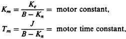
Based on these relationships, the values of Km and Tm for the overall combination of servomotor, gear train, and load inertia can now be obtained. To do this, it is assumed that the damping factor B in Eq. (3.101) is zero (it is usually negligible compared with the motor damping Kn):
where Kml denotes the value of Km referred to the output shaft. This indicates that the system gain is reduced by a factor of N. Furthermore,
This indicates an increase in the servomotor time constant due to the added load inertia. Therefore, the net effect of the gear reduction and the load inertia has been to reduce Km by a factor of N, and to increase the time constant by the added term JL/N2Knm. Therefore, the transfer function of the two-phase ac servomotor with a gear reduction N and a load inertia JL is given by
Now let us approach the problem by referring all quantities to the motor shaft and check the result. For this case, the only two factors that have to be considered are the effect of the gear reduction N and the load inertia JL. As we have just observed, the effect of the gear reduction N is basically a loss in system gain N. Therefore, it must be treated as an element having a transfer function 1/N. What about the load inertia JL? Let us reconsider Eq. (3.112) and reflect the load inertia to the servomotor:
![]()
where JLr is the load inertia referred to the motor shaft. Therefore,
![]()
This indicates that the load inertia at the motor shaft is reduced by a factor of N2. We are now ready to determine the values of Km and Tm of the servomotor and gear-reduction combination. As before, B is assumed to be zero. Therefore,
and
Observe the agreement between Eqs. (3.115) and (3.118) and between Eqs. (3.116) and 3.119).
The results derived here can easily be extended to multimesh gear trains as illustrated in Figure 3.20. In this figure, a two-mesh system is illustrated, and the inertia of the respective shafts and gearing combinations are indicated as J1, J2, and J3. It is left as an exercise to the reader to show that the equivalent inertia reflected to the input (motor) shaft is
![]()
and the equivalent inertia reflected to the output shaft is given by
![]()

Figure 3.20 A multimesh gear train.
Before leaving the subject of gear ratios, the question is posed as to what is the optimum gear ratio for a given motor and load configuration? This problem can be answered by reconsidering the servomotor, gear train, and load configuration ilustrated in Figure 3.19. The torque developed by the motor (at the motor shaft) in accelerating its own inertia, Jm, and the load inertia, JL, through the gear ratio N, is given by
where αl(t) represents the maximum required acceleration of the load. Equation (3.120) represents the developed torque at the motor shaft with the load inertia component appropriately reflected to it. In order to find the optimum gear ratio N which will minimize the required motor torque and therefore the size of the motor, Eq. (3.120) is differentiated with repect to N and is set equal to zero:

Therefore, the gear ratio required to minimize the motor torque is given by
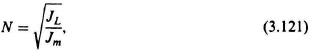
where the gear ratio N is the square root of the ratio of the load to motor inertias. Equation (3.121) may also be interpreted from the viewpoint that the value of motor inertia for minimum motor torque required is given by
Therefore, Eq. (3.122) states that the motor torque is minimized when the motor and load inertias are equal when referred to a common shaft.
Note that this result assumes that the only factor that is important is acceleration of the load. If a maximum load velocity is specified and the motor can only reach a given maximum velocity, the choice of optimum gear ratio is different.