6.7.  BODE-DIAGRAM APPROACH

The Bode-diagram approach [8] is one of the most commonly used methods for the analysis and synthesis of linear feedback control systems. This method, which is basically an extension of the Nyquist stability criterion, has the same limitations and uses as the Nyquist diagram. The presentation of information in the Bode-diagram approach, however, is modified to permit relatively quick determinations of the effects of changes in system parameters without the laborious calculations associated with the Nyquist diagram.

Table 6.6. MATLAB Program for Converting from the Transfer Function to the State-Space Form

num = [0  0  0  1];
den = [1  2  1  0];
[A, B, C, D] = tf2ss(num,den)
A=
−2   −1    0
1     0    0
0     1    0
B =
1
0
0
C =
0  0  1
D =
0

Table 6.7. MATLAB Program for Determining the Nyquist Diagram from the State-Space Form

A = [−2    −1    0; 1    0;    0; 0    1    0]; B = [1;0;0] C = [0    0    1]; D = [0]; nyquist(A,B,C,D) axis([−1.8   0   −2.5   2.5]) grid title(‘Nyquist plot of G(s) ∗ H(s) = 1/[s ∗ (s + 1)^2]’)

The Nyquist diagram gives the amplitude and phase of the open-loop transfer function G(s)H(s) as s traverses a contour that encloses the right half-plane. As s traverses the positive imaginary axis, it has the value of real frequency ω, and the plot corresponds to G(jω)H(jω). We can illustrate the same amount of information by means of two diagrams which have ω as a common axis. These two diagrams, illustrated in Figure 6.18, are usually referred to as the Bode diagram. The magnitude of G(jω)H(jω) is 20 log₁₀ G(jω)H(jω); the unit used to represent this is decibels (dB). For this logarithmic representation, the amplitude and phase curves are drawn on semilog paper with the log scale used for frequency. The linear scales are used for magnitude in decibels, and phase degrees. The number of cycles needed for the frequency range is based on the frequency range of the problem being analyzed. It is important to emphasize that the Bode diagram provides information only of s corresponding to the positive imaginary axis, and therefore represent the frequency response.

Let us consider the system illustrated in Figure 6.19. It is assumed that the input r(t) is a sinusoidal waveform ω and unity amplitude given by

Figure 6.18   Typical Bode diagram.

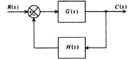
Figure 6.19   Representative feedback control system.

Assuming a linear system, the output would have the general form

where a = gain of system and = phase shift of the system. Let us represent the system transfer function as

Here H(jω) is a complex function which can be represented by an amplitude a(jω) and a phase shift of (jω). In the Bode-diagram approach, the amplitude is expressed in decibels and is plotted versus frequency on semilogarithmic graph paper. The amplitude, in decibels, is given by

The phase shift (jω) is conventionally expressed in degrees.

By introducing the logarithm concept, the tedious process of multiplying two complex numbers is simplified to one of addition. For example, let us consider two complex numbers: G_a(jω) and G_b(jω). The logarithm of the product of two complex quantities,

and

is given by

Equation (6.77) illustrates that the logarithm of the product of two complex numbers is the sum of the logarithms of the magnitude components. The total phase equals the sum of the individual phase-angle components. A minus appears before the phase contribution term in Eq. (6.77) because the individual phase components were assumed to be negative in Eqs. (6.75) and (6.76). In addition, Eq. (6.77), shows that the logarithm of the magnitude and phase components, respectively, are separate functions of the common parameter ω and can be sketched separately, as was shown in Figure 6.18.

Bode’s theorems are presented in Chapter 7 when we discuss the Bode-diagram approach for the design of feedback control systems in order to meet certain specifications. In this chapter, however, it is important to emphasize the fact that the Bode-diagram approach applies primarily only to minimum-phase systems. The basic definition of a minimum-phase system [9] is a system whose phase shift is the minimum possible for the number of energy storage elements in the network. A system is denoted as being minimum phase if all its poles and zeros lie in the left half of the s-plane. If at least one of its poles or zeros lies in the right half-plane, then the system is denoted as being a nonminimum-phase system. This definition restricts the poles and zeros of minimum-phase systems to the left half of the complex-plane. A little thought indicates that when we specify either the amplitude or phase of a minimum-phase system, we have also automatically specified the other. This concept is the basis of one of Bode’s theorems. However, the Bode diagram can be applied to nonminimum-phase systems if we know where the nonminimum-phase characteristics come from.

Understanding the basic concepts of the Bode diagram, let us now gain the facility for constructing them. The laborious procedure of plotting the amplitude and phase of G(jω)H(jω) by means of substituting several values of jω is not necessary when drawing the Bode diagram, because we can use several shortcuts. These shortcuts are based on simplifying the approximations that allow us to represent the exact, smooth plots with straight-line asymptotes. The difference between actual amplitude characteristics and the asymptotic approximations is only a few decibels. Now we shall demontrate the application of this approximating technique to seven common, representative transfer functions: a constant, a pure integration, a pure differentiation, a simple phase-lag network, a simple phase-lead network, a quadratic phase-lage network and a time-delay factor. The basic concepts illustrated are then used to draw the Bode diagram of the transfer function for representative systems. We will then show how the Bode diagram can be obtained using MATLAB in Section 6.8, and other commercial programs presented in Section 6.21.

A.  Bode Diagram of a Constant

Using the definition of Eq. (6.74), the logarithm of a constant K, or 1/K, where K > 1, is given by

The corresponding phase angle of a constant is 0°. Figure 6.20 illustrates the Bode diagram of a constant.

Figure 6.21 provides an easy way to obtain a decibel value for different numbers. Observe from this conversion line that ratios of two (an octave) corresponds to 6 dB; ratios of ten (decade) correspond to 20 dB. In addition, observe that the reciprocal of a number differs form its value only by the sign:

B.  Bode Diagram of a Pure Integration

The Bode diagram of a pure integration

Figure 6.20   Bode diagram of a constant.

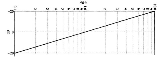
Figure 6.21   Conversion curve between numbers and decibels.

can be obtained by taking the logarithm, yielding

Figure 6.22 illustrates the Bode diagram of a pure integration. Notice that the resulting amplitude curve is linear when the amplitude is plotted on a linear scale and the frequency is plotted on a logarithmic scale. The slope of the amplitude characteristic is a constant and equals −20 dB/decade. A slope of −20 dB/decade also corresponds to a slope of −6 dB/octave. The phase characteristic for the pure integration is constant and equals −90°.

C.  Bode Diagram of a Pure Differentiation

The Bode diagram of a pure differentiation

can be obtained in a manner similar to that used for the pure integration. The major differences are that the amplitude characteristics now have a positive slope and the phase characteristic is positive. Figure 6.23 illustrates the Bode diagram of a pure differentiation.

Figure 6.22   Bode diagram of a pure integration.

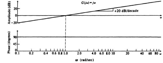
Figure 6.23   Bode diagram of a pure differentiation.

D.  Bode Diagram of a Simple Phase-Lag Network

A phase-lag network produces a phase lag that is a function of frequency. The transfer function of such a network is given by

The Bode diagram for this transfer function can be obtained as follows:

Figure 6.24 illustrates the Bode diagram of a simple phase-lag network. The dashed portion of the amplitude characteristic represents the exact plot, and the heavy-line segments represent the straight line asymptotic approximation. They differ by a maximum of 3 dB at ω/a = 1 and by 1 dB an octave away.

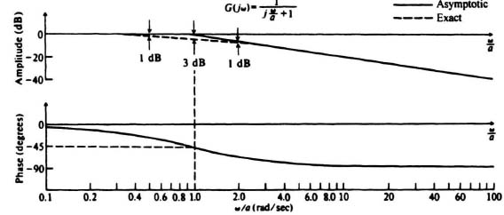
Figure 6.24   Bode diagram of a simple phase-lag network.

The asymptotic approximation can be drawn quite easily. For example, when ω/a is much less than unity, the imaginary component is very much smaller than the real component (unity), and the imaginary component can be neglected. Therefore,

When ω/a is much greater than unity, the imaginary component is much greater than the real component (unity) and the real component may be neglected.
Therefore

Equation (6.87) is very similar to the amplitude characteristic of a pure integrator, given by Eq. (6.82), and has a slope of −20 dB/decade. At ω/a = 1, the two asymptotes join each other. This frequency (ω = a) is referred to as the break or comer frequency. Ordinarily, the straight-line asymptotic approximation is accurate for most applications. If further correction is needed, the exact curve can be obtained from the approximate curve by using the following corrections: −1 dB at ω/a = 0.5 and 2; −3 dB at ω/a = 1. Additional corrections can be obtained from Figure 6.25 which illustrates the corrections in decibels as a function of a.

The phase shift produced by the simple phase-lag network can be obtained from the expression

The phase shift at the break frequency is −45°; at ω = 0 it is 0°; at ω = ∞ it is −90°. Notice that this phase-lag network is a minimum-phase network, because the pole is in the left half-plane, and it has the minimum phase shift possible for the number of energy storage elements in the network (one).

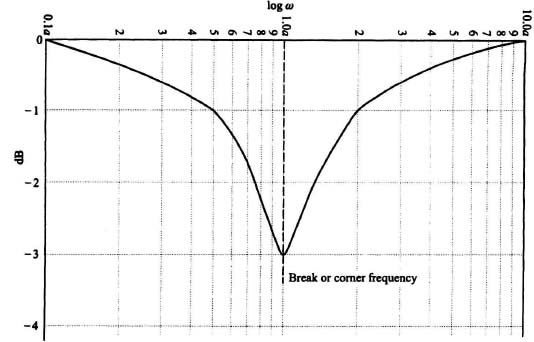
Figure 6.25   Errors is the asymptotic plot for the simple phase-lag network a/(jω + a).

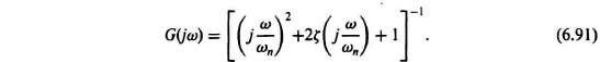
E.  Bode Diagram of a Simple Phase-Lead Network

The Bode diagram of a simple phase-lead network

can be obtained in a manner similar to that used for the simple phase-lag network. The major differences are that the amplitude characteristic has a positive slope, and the phase characteristic has a positive (phase-lead) value. Figure 6.26 illustrates the Bode diagram of a simple phase-lead network.

F.  Bode Diagram of a Quadratic Phase-Lag Network

Let us consider the second-order quadratic, phase-lag transfer function given by

or

The Bode diagram for this transfer function can be obtained as follows:

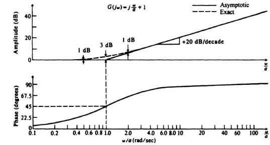
Figure 6.26   Bode diagram of a simple phase-lead network.

Figures 6.27 and 6.28 illustrate the Bode diagram of the quadratic phase-lag network for various values of damping ratio, ξ. In Figure 6.27, the dashed portion of the amplitude characteristic represents the straight-line asymptotic approximation and the heavy-line portions represent the exact plot. For ζ = 1, the two curves differ by a maximum of 6.02 dB at ω/ω_n equal to unity.

Figure 6.27   Amplitude portion of Bode diagram for a quadratic phase-lag network.

Figure 6.28   Phase portion of Bode diagram for a quadratic phase-lag network.

The asymptotic approximations can be drawn quite simply. For example, when ω/ω_n is much less than unity, the imaginary component is very much smaller than the real component, and the imaginary component can be neglected. Therefore,

When ω/ω_n is much greater than unity, the dominant term is

This indicates that the slope of the straight-line asymptotic approximation for ω/ω_n 1 is twice that of a phase-lag network. The difference between the approximate curve and the exact curve depends on the damping factor ζ. Similar analysis indicates the phase shift possible is twice that of the simple phase-lag network (e.g., −180°). The phase shift characteristics are shown in Figure 6.28.

G.  Bode Diagram of a Time-Delay or Transportation Lag Factor

The time-delay factor [10] occurs in systems which are characterized by the movement of mass that requires a finite time to pass from one point to another. The transfer function of a pure time-delay or transportation lag factor, without attenuation, is given by

The delay factor e^−jωT results in a phase shift

which has to be added to the phase shift resulting from the rest of the system. Observe that the magnitude of the time-delay or transportation lag factor is always unity and, therefore, does not affect the magnitude characteristics. Figure 6.29 illustrates the Bode diagram of the pure time-delay factor on a logarithmic scale.

Time-delay or transportation lag factors are very common in hydraulic, pneumatic, thermal, chemical, and manual (human in the loop) control systems. They have nonminimum-phase characteristics with very large phase lags and no attentuation at high frequencies.

H.  Bode Diagram of a Composite Transfer Function—Example 1

Let us next apply the basic concepts developed in this section for the transfer function of a simple system. Consider a unity-feedback system whose open-loop transfer function is given by

This system contains a gain of 10, a pure integration, and a pole term whose break frequency is at 10 rad/sec. The step-by-step procedure for drawing this Bode diagram is as follows. We will describe graphical techniques for drawing the Bode diagram in this section. Working computer programs are provided in Section 6.9. Commercially available computer programs for obtaining the Bode diagram are presented in Section 6.8. The MATLAB program, which is described in Section 6.8, was used for drawing the actual Bode diagrams for Examples 1 (Figure 6.30), 2 (Figure 6.31), 3 (Figure 6.33), and 4 (Figure 6.34) of this section. These Bode diagrams are contained in the M-files (that are part of my Modern Control System Theory and Design Toolbox) that can be retrieved free from The MathWorks, Inc. anonymous FTP server at ftp://ftp.mathworks.com/pub/books/shinners.

Figure 6.29   Bode diagram of a pure time-delay factor.

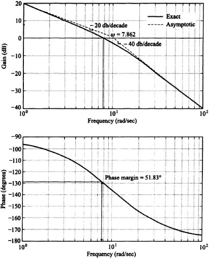
Step 1. We will plot the amplitude characteristics first. A frequency is picked at least 1 decade below the lowest break frequency and the gain and slope are fixed at that frequency. In this example, that frequency is 1 rad/sec, where the pole term is approximated as one [see Eq. (6.86)]. Therefore, the composite gain is 10 (or 20 dB) and the slope is −20 dB/decade due to the pure integration.

Step 2. The slope of −20 dB/decade is continued until the first break at 10 rad/sec occurs, where we add another −20 dB/decade and make the slope −40 dB/decade, which continues to infinity. The result is shown in Figure 6.30. Notice that if we use the straight-line asymptotic approximation (dashed line in Figure 6.30), a gain crossover frequency (defined as the frequency where the G(s)H(s) curve crosses the 0-dB line) of 10 rad/sec occurs where a break frequency also occurs. Therefore, we must correct the straight-line asymptotic approximation by the 3-dB error at the break frequency as shown in Figure 6.30 (solid line). Therefore, the actual gain crossover frequency is at 7.862 rad/sec. Whenever a break frequency occurs at the gain crossover frequency, or close to it, we must use the corrected curve to determine the actual gain crossover frequency. Otherwise, large errors will occur in determining the phase margin from the Bode diagram (see Step 4).

Figure 6.30   Bode diagram for system whose open-loop transfer function is

Step 3. The phase characteristic is obtained by adding the phase of each component of the composite transfer function. The gain factor contributes zero degrees of phase shift (see Figure 6.20). The pure integration provides a constant phase shift of −90° at all frequencies (see Figure 6.22). The pure integration provides a constant phase shift of −90° at all frequencies (see Figure 6.22). The pole term provides a phase contribution of −tan⁻¹ 0.1ω (see Eq. (6.88). Therefore, in this example, the composite phase is computed from

Step 4. The phase and gain margins, defined in Eqs. (6.67) and (6.69) for the Nyquist diagram, can also be determined from the Bode diagram in this step. Let us determine next how this can be accomplished.

I.  Relationship Between Bode and Nyquist Diagrams

At this point in the development of the Bode diagram, it is appropriate to relate the Nyquist stability criterion to the Bode amplitude and phase diagrams. When we discussed the Nyquist diagram, the degree of stability was defined in terms of the phase and gain margins present (see Figure 6.14). This can easily be related to the Bode diagrams by making use of the following two facts.

1. The unit circle of the Nyquist diagram transforms into the unity or 0-dB line of the amplitude plot for all frequencies.
2. The negative real axis of the Nyquist diagram transforms into a negative 180° phase line for all frequencies.

Therefore, the phase margin can be determined on the Bode diagram by determining the phase shift present when G(jω)H(jω) crosses the 0-dB line. The gain margin can be obtained on the Bode diagram by determining the gain present when G(jω)H(jω) crosses the −180° line.

Returning to Step 4 of Example 1, the Bode diagram which is illustrated in Figure 6.30, the gain crossover frequency is at 7.862 rad/sec where the phase shift is 128.17° (this corresponds to the θ of Figure 6.14), and the resulting phase margin is 51.83° (this corresponds to the γ of Figure 6.14). Because this example never reaches −180° (except at ω = ∞), its gain margin is infinity. Therefore, this system is stable.

The values of gain crossover frequency, phase, and gain margins determined in this section and the rest of the book where the Bode diagram is applied, use the function “margins,” which is part of my Modern Control System Theory and Design Toolbox. It calculates their values based on their definitions, analytically and very accurately, rather than using graphical techniques. The disk that contains my tool-box can be retrieved free from The Math Works, Inc. anonymous FJP server at ftp://ftp.mathworks.com/pub/books/shinners.

J.  Bode Diagram of a Composite Transfer Function—Example 2

For the second example, let us consider a unity-feedback control system whose forward transfer function is given by

This system contains a gain, a pure integration, and a double pole term whose break frequency is at 10. The Bode diagram of this system, shown in Figure 6.31, was also obtained using MATLAB and is contained in the M-file that is part of my Modern Control System Theory and Design Toolbox.

The gain and slope at ω = 1 rad/sec (two decades below the lowest and only break frequency) is fixed, where the gain is 40 dB and the slope is −20dB/decade due to the pure integration. This slope is continued using the straight-line approximation (dashed line in Figure 6.31) to the double break at 10 rad/sec. There, we add −40 dB/decade to the slope due to the double pole, and the straight-line approximation continues at a slope of −60 dB/decade thereafter. Because there is a break at the gain crossover frequency (a double one in this example), we must again correct for this to find the actual gain crossover frequency. The solid-line curve in the amplitude plot of Figure 6.31 indicates that the actual crossover frequency is at 6.825 rad/sec (not 10 rad/sec). The composite phase is computed from

The phase shift at 6.825 rad/sec is 158.61°. Therefore, the phase margin is 21.39°. At a frequency of 10.02 rad/sec, the phase shift is −180°. This frequency is defined as the phase-crossover frequency. Therefore, the gain margin for this system is 6.039 dB as indicated in Figure 6.31. Therefore this system is stable.

K.  The Phase-Shift Scale

For, quick approximate phase-shift calculations, the phase characteristics can easily be determined using superposition of the individual characteristics of each component using the phase-shift scale shown in Figure 6.32. This scale, which can easily be derived from the tangent relationship, illustrates the effect on the resultant phase shift occurring at frequency ω for a first-order factor, due to a break frequency occurring at ω₀. For example, at ω/ω₀ = 5, the phase shift contributed by the break occurring at ω₀ = 1 is 78.7°, whereas at ω/ω₀ = 0.2 the phase shift contributed by this break is only 11.3°.

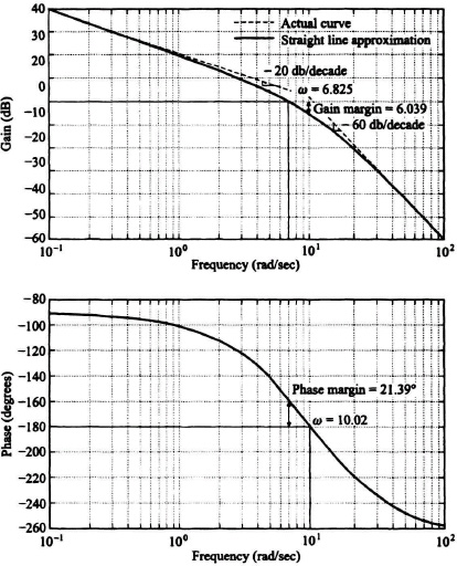
Figure 6.31   Bode diagram for system whose open-loop transfer function is

                                                              

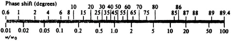
Figure 6.32   Phase-shift scale illustrating the effect on the resultant phase shift occurring at ω due to a break at ω₀.

H.  Bode Diagram of a Composite Transfer Function—Example 3

Let us next apply the basic notions developed in this section for the transfer function of a unity-feedback system whose forward transfer function is given by

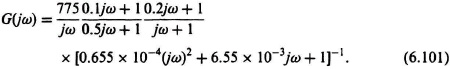
This transfer function contains a pure integration, two simple phase lags, two simple phase leads, and a quadratic phase-lag network. Each of these characteristics has previously been considered individually. The simplest procedure for plotting the amplitude characteristic for the entire transfer function is to start by locating one point, ω = 0.1, which is one decade below the lowest break (ω = 1). At the same time, the slope at ω = 0.1 is determined. For the problem at hand, at ω = 0.1,

Equation (6.102) indicates that the gain of the straight-line asymptotic curve is 7750 (77.8 dB) and the slope is −20 dB/decade at ω = 0.1.

The next step is to locate all the break frequencies (frequencies at which the slopes change because a real or imaginary component starts or stops dominating). The break frequencies for this transfer function are at ω = 1 (−20 dB/decade to −40dB/decade); ω = 2 (−40 dB/decade to −60 dB/decade); ω = 5 (−60 dB/decade to −40 dB/decade); ω = 10 (−40 dB/decade to −20 dB/decade); ω = 123.8 (−20 dB/decade to −60 dB/decade). The corresponding phase characteristics can most easily be determined using superposition of the individual phase characteristics of each component as was illustrated in the previous two examples.

Figure 6.33 illustrates the composite Bode diagram for the transfer function given by Eq. (6.101). Notice that the peaking due to the quadratic phase-lag component occurs at ω_n = 123.8, and corresponds to ζ = 0.405. The Bode diagram was drawn using MATLAB (see Section 6.8) and is contained in the M-File that is part of my Modern Control System Theory and Design Toolbox and can be retrieved free from The MathWorks, Inc. anonymous FJP server at ftp://ftp.mathworks.com/pub/books/shinners. The straight-line asymptotic approximations (dashed line) were added for illustrative purposes. The results of this Bode diagram show a gain crossover frequency of 34.33 rad/sec, a phase margin of 56.74°, and a gain margin of 9.622 dB (the phase crossover frequency where the phase is −180°, occurs at 118.7 rad/sec).

M.  Bode Diagram of a Composite Transfer Equation Containing a Time-Delay Factor—Example 4

As a fourth example of a Bode diagram, let us consider a unity-feedback system whose forward transfer function is given by

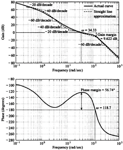
Figure 6.33   Composite Bode diagram for a unity-feedback system whose G(jω) is given by Eq. (6.101).

This transfer function contains a pure integration, one pole, one zero, and a time delay factor. This represents the transfer function in a steel mill, and the time-delay factor is caused by the finite time it takes the steel to move from one point to another. In this system, a motor adjusts the separation l of two rolls so that the thickness error of the steel is minimized. If the steel is traveling at a velocity v of 10ft/sec, and the nominal separation d is 1 ft, then the time delay between the roll thickness measurement and thickness adjustment is given by

The overall transfer function G(jω), given by Eq. (6.103), relates the transfer function of the system error, defined as system error = desired thickness − actual thickness, and the output which represents the actual thickness.

Each of the other characteristics in Eq. (6.103) has been previously considered separately. Again, our procedure for plotting the amplitude characteristics is to start by finding the gain and slope at a frequency below the lowest break (ω = 2). Therefore, we will perform the calculation at ω = 0.1. For this problem, the amplitude of G(jω) at ω = 0.1 is

Equation (6.104) indicates that the gain is 200 (46 dB) and the slope is −20 dB/decade at ω = 0.1. The break frequencies occur at ω = 2, where the slope changes from −20 dB/decade to −40 dB/decade, and ω = 5 when the slope changes from −40 dB/decade to −20 dB/decade. The corresponding phase characteristic can be readily determined using superposition of the individual phase characteristics of each component. Figure 6.34 illustrates the composite Bode diagram for the transfer function given by Eq. (6.103). For interest, the phase characteristic is illustrated with and without the time-delay factor. Observe from this curve that the gain crossover frequency is 8.967 rad/sec and the phase margin of the system without the time-delay factor is 73.42°. For this case, the gain margin is infinity because the phase never reaches −180°. However, with the time-delay factor in the system, the phase margin drops to 22.04°, the gain margin becomes 4.16 dB (the phase crossover frequency equals 13.65 rad/sec), and the system has a smaller margin of stability than before. The control-system engineer should always give particular attention to time-delay factors and avoid them if possible, because they produce a phase lag and decrease the phase margin. The Bode diagram was drawn using MATLAB (see Section 6.8). The straight-line asymptotic approximation (dashed line) was added for illustrative purposes.

Figure 6.34   Composite Bode diagram for a unity-feedback system where G(jω) is given by Eq. (6.103).

The Bode-diagram method has the very practical virtue that the amplitude and phase frequency response can easily be measured in the laboratory. The relative ease of synthesizing feedback control systems with the Bode-diagram approach is further demonstrated in Chapters 7, 8, 9, and 12.