6.10.  NICHOLS CHART

The Nichols chart [21] is a very useful technique for determining stability and the closed-loop frequency response of a feedback system. Stability is determined from a plot of the open-loop gain versus phase characteristics. At the same time, the closed-loop frequency response of the system is determined by utilizing contours of constant closed-loop amplitude and phase shift which are overlaid on the gain-phase plot.

In order to derive the basic Nichols chart relationships, let us consider the unity-feedback system illustrated in Figure 6.45. The closed-loop transfer function is given by

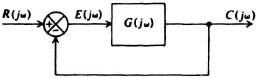
Figure 6.45   Block diagram of a simple feedback control system.

or

where M(ω) represents the amplitude component of the transfer function and α(ω) the phase component of the transfer function. The radian frequency at which the maximum value of C(jω)/R(jω) occurs is called the resonant frequency of the system, ω_p, and the maximum value of C(jω)/R(jω) is denoted by M_p. For the system illustrated in Figure 6.45, we would expect a typical closed-loop frequency response to have the general form shown in Figure 6.46.

From Section 4.2 we know that a small margin of stability would mean a relatively small value for ζ and a relatively large value for M_p. This can be further clarified if we examine the Nyquist diagrams illustrated in Figure 6.47. Notice that M(ω) is much less than unity for the case of a system having a large degree of stability, as shown in part (a) of the figure. In contrast, M(ω) is much greater than unity for the case of a system having a very small degree of stability, as shown in part (b) of the figure. We next develop the Nichols-chart contours in the complex plane in order to be able to determine M_p and ω_p quantitatively for a feedback control system.

Reconsidering the basic relationships of the unity-feedback control system illustrated in Figure 6.45, let us represent the complex vector G(jω) by an amplitude and phase as follows:

Substituting Eq. (6.114) into the system transfer function, as given by Eq. (6.112), we obtain

Figure 6.46   A typical closed-loop frequency-response curve for the system shown in Figure 6.45.

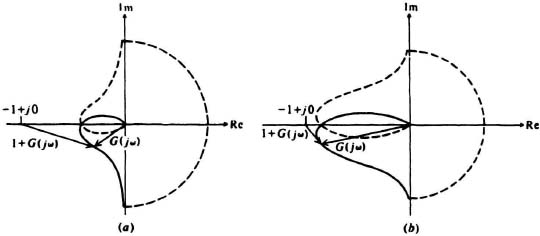
Figure 6.47   Qualitative stability comparison of two systems illustrating corresponding values of M(ω). (a) Stable system with large degree of stability:

                                                                   

(b) Stable system with very small degree of stability:

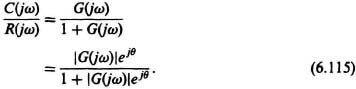
Dividing through by |G(jω)|e^jθ, we obtain

Using the trigonometric relationship for the exponential term, we obtain the expression

The expression of Eq. (6.117) has a magnitude of M(ω) and a phase angle α(ω) which are given by

A detailed plot of G in decibels versus θ in degrees, with M and α as parameters, known as the Nichols chart, is illustrated in Figure 6.48. Notice the symmetry of these curves about the −180° and 0 dB point.

The stability criterion for the Nichols chart is quite simple, because the −1 + j0 point of the Nyquist diagram corresponds to the 0-dB, −180° point of Figure 6.48. Therefore, for minimum-phase systems, the phase margin and gain margin can be determined.

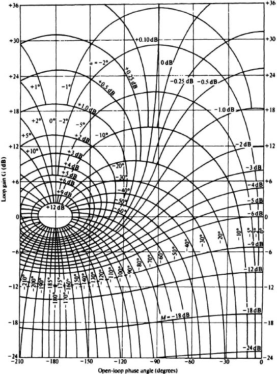
Figure 6.48   Nichols chart.

The Nichols chart can be used for the analysis and/or synthesis of a feedback control system. For analysis, we can use the Nichols chart to obtain the closed-loop frequency response from the Bode diagram and determine the maximum value of peaking M_p and the frequency at which it occurs, ω_p. From a synthesis viewpoint, we can use the Nichols chart to meet certain requirements as to the values of M_p and ω_p. We demonstrate the use of this method as a total for analysis in this section. Its value as a tool for synthesis is illustrated in Section 7.8 of Chapter 7.

Let us determine the closed-loop frequency response for the third-order feed-back control system which is illustrated in Figure 6.49. Specifically, we are now interested in obtaining the values of M_p and ω_p using the Nichols chart. They can be obtained by first drawing the Bode diagram as shown in Figure 6.50. Then, for each value of ω, the magnitude and phase of G(jω) are then plotted onto a Nichols chart as shown in Figure 6.51a. The Bode diagram and Nichols chart were obtained using MATLAB, and are contained in the M-file that is part of my MCSTD Toolbox and can be retrieved free from The MathWorks, Inc. anonymous FTP server at ftp://ftp.mathworks.com/pub/books/shinners. It indicates a phase margin of 27.7° and a gain margin at 8.175 dB which agrees with the values obtained from the Bode diagram of Figure 6.50. The intersections of G(jω) with M(ω) on the Nichols chart give the closed-loop response from which M_p and ω_p can be obtained. The resulting response, shown in Figure 6.51b, indicates a value of M_p = 6.758 dB (2.2) and ω_p = 8.989 rad/sec. This too was obtained using MATLAB. It is important to note that the use of MATLAB and the MCSTD Toolbox permits one to obtain the Nichols chart directly without having to first obtain the Bode diagram.

In practice, a value of M_p = 2.2 is a little too high. Usually, M_p is chosen somewhere between 1.0 and 1.4 (see Section 7.8). The technique of compensation of this system utilizing the Nichols chart is illustrated in Section 7.8 of Chapter 7. Let us here, however, indicate how the constant M loci on the Nichols chart may be used to limit M_p to some maximum value, say 2.2 dB (1.3). Because the interior of the M = 2.2 dB locus consists entirely of constant-magnitude loci which represent M greater than 2.2 dB, we must confine the Nichols locus to the exterior of the M = 2.2 dB locus. The system illustrated in Figure 6.49 is compensated, to meet certain maximum requirements of M_p, in Section 7.8 of Chapter 7 utilizing the Nichols chart.

The values of ω_p and M_p determined in this section and the rest of the book where the Nichols chart is applied, uses the function “wpmp” which is part of my MCSTD Toolbox. It calculates ω_p and M_p analytically and very accurately rather than using graphical techniques. My toolbox is available to the reader free, and can be retrieved from The Mathworks, Inc. anonymous FTP server at ftp://ftp.mathworks.com/pub/books/shinners.

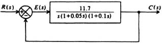
Figure 6.49   A third-order feedback control system.

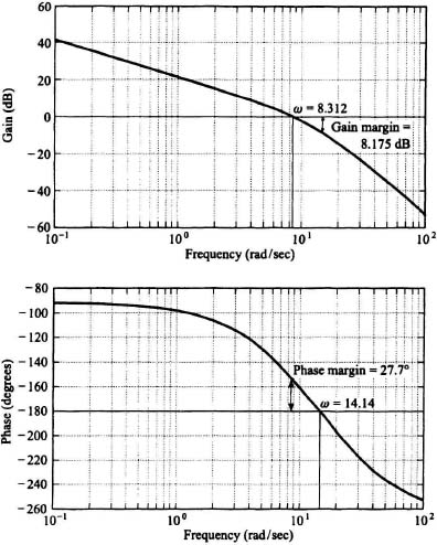
Figure 6.50   Bode diagram for the system shown in Figure 6.49, where

                                                                   .

In the following section, 6.11, the procedure for obtaining the Nichols chart using MATLAB is provided. This is of great assistance to the control-system engineer in obtaining very powerful results with a few MATLAB statements.