2.25.  OBTAINING THE TRANSIENT RESPONSE OF SYSTEMS USING MATLAB [6]

In the previous section, an algorithm (Eq. 2.248) was developed for obtaining the time response of a control system based on a knowledge of the P and B matrices, and a digital computer program was written in Fortran and applied to obtain the unit response for the control system illustrated in Figure 2.29. In this section, the relatively simple procedure for obtaining transient responses of control systems using MATLAB will be provided.

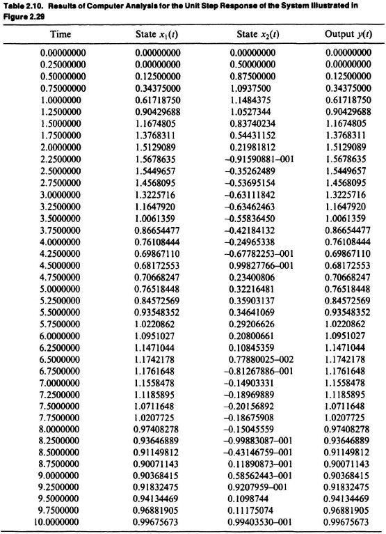
Figure 2.35   Response of the system shown in Figure 2.29 to a unit step input for sampling times of 0.05–0.5 sec (a). and a comparison of the case of a 0.05-sec sampling time with the theoretical response (b).

The MATLAB commands, found in the Control System Toolbox and The Student Edition of MATLAB, for obtaining the unit step response of a control system are as follows:

(a)  If the numerator (num) and denominator (den) of a closed-loop system are known in transfer function form:

step(num,den)

If the user wishes to supply the time t at which the step response will be computed at regularly spaced times, the following command is used:

step(num,den, t).

The time vector is automatically determined when t is excluded from the command.

As an illustration for obtaining the transient response to a unit setp input, let us reconsider the problem analyzed in the previous section where we obtained the unit step response to the control system illustrated in Figure 2.29. The closed-loop transfer function of the control system illustrated in Figure 2.29 is given by

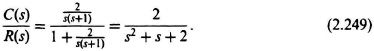
Therefore, the MATLAB program for obtaining the unit step response for this control system is given by the MATLAB Program in Table 2.11.

The resultant transient response is illustrated in Figure 2.36. Observe that it is the same as the theoretical curve illustrated in Figure 2.35b.

(b)  If the state-space form (including A (or P), B, C (or L), and D) are known:

step(A,B,C,D).

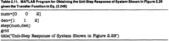
Figure 2.36   Unit step response of system shown in Figure 2.29 obtained using MATLAB Program in Table 2.11.

If the user wishes to supply the time t at which the response will be computed at regularly spaced times, use the following command:

step(A,B,C,D,t).

If the control system has multiple inputs, the command

step(A,B,C,D,iu)

or

step(A,B,C,D,iu,t)

produces a step response from the single input “iu” specified to all the outputs of the system. The scalar, iu, is an index into the inputs of the system and specifies which input is to be used for the response.

These “step” commands do not result in a plot on the screen. Therefore, it is necessary to use the “plot” command in order to obtain the graphical transient response.

As an illustration for obtaining the transient response to a unit step input from knowledge of the state-space form, we will reconsider the same problem analyzed previously in this section.

The corresponding phase-variable canonical equations for the control system shown in Figure 2.29 are as follows:

Therefore, the matrices A (or P), B, C (or L), and D are given by:

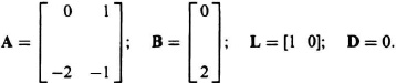
The resulting MATLAB program used to obtain the unit step response from knowledge of the phase variables canonical form is given in Table 2.12.

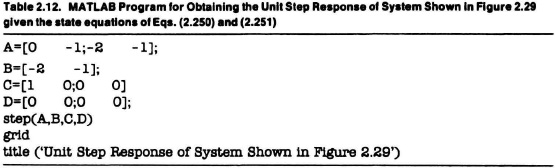
The resultant transient response as illustrated in Figure 2.37. Observe that it is the same as that shown in Figure 2.36, and that shown as the theoretical curve in Figure 2.35b.