
8.11. AN INTRODUCTION TO H∞ CONTROL CONCEPTS [16, 17]
In the presentation of this book, the classical frequency-domain approach and the modern state-variable time-domain approach have been presented in parallel. It has been shown that they complement each other. Prior to the 1960s, the frequency-domain approach predominated. With the advent of the space race, the availability of practical digital computers, modem optimal control theory, and the state-variable approach in the early 1960s, the pendulum swung to the time-domain approach. The 1960s and 1970s saw an abundant amount of work performed on applying modern optimal control theory, which is presented in Chapter 11 in this book. In the early 1980s, a new technique has emerged known as H∞ control theory which combines both the fequency- and time-domain approaches to provide a unified answer. Zames is given credit for its introduction with his paper in the IEEE Transactions on Automatic Control [16]. The H∞ approach has dominated the trend of control-system development in the 1980s and 1990s. A complete treatment of the subject of H∞ is complex, and beyond the scope of this book. However, we can expand the concepts of robustness (introduced in Section 8.10) and sensitivity (introduced in Chapter 5), together with the frequency and state-variable domain techniques presented in this book to introduce the basic concepts of H∞ control theory and apply it to some simple problems. This is the objective of this and the following sections.
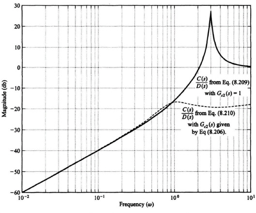
Figure 8.28 Frequency response of the disturbance suppression transfer functions defined in Eqs.(8.209) and (8.210).
A. Sensitivity of Control Systems Containing Disturbances and Measurement Noise
Let us extend our understanding of sensitivity developed in Chapter 5 to the control system illustrated in Figure 8.29 which contains a disturbance U(s) and feedback sensor measurement noise N(s). Although noise is a stochastic process, we will assume in this analysis that it can be represented as a deterministic process. This initial analysis will focus on the single-input single-output (SISO) system shown in Figure 8.29 which contains a disturbance U(s) and feedback sensor measurement noise N(s). We will then discuss the extension of these results to multiple-input multiple-output (MIMO) systems.
Using Mason’s theorem, we can write the following relationship for the output C(s) by inspection of Figure 8.29:
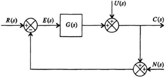
Figure 8.29 Control system containing a disturbance U(s) and sensor measurement observation noise N(s).
We can also use Mason’s theorem to write the following relationship for the control-system error E(s) by inspection of Figure 8.29:
From the analysis in Section 5.3 on sensitivity, we know that the sensitivity of the transfer function C(s)/R(s) to changes in G(s) for the control system shown in Figure 8.29 is given by the following expression:
It is interesting to observe that this sensitivity is also the transfer function from U(s) to −E(s):
In the MIMO case, the sensitivity function in Eq. (8.213) is modified so that G(s) becomes the matrix of transfer functions between the inputs and the outputs, and the value of 1 is replaced with the identity matrix.
The transfer function C(s)/R(s) of the control system shown in Figure 8.29 is given by the following:

This expression is also known as the complementary sensitivity function which is defined as follows:
It is very important to recognize that the sum of the sensitivity function given by Eq. (8.213), and the complementary sensitivity function given by Eq. (8.216) equals one:
We can express the error function E(s) in Eq. (8.212) in terms of the sensitivity function. Let us assume that the feedback sensor measurement noise is zero. Therefore, substituting Eq. (8.213) into Eq. (8.212), we obtain the following:
Equation (8.218) is a very important relationship because it states that we should make the sensitivity function S small to make the control system error E(s) small. In addition, we know that since Eq. (8.213) represents the sensitivity function as well as the transfer function between U(s) and −E(s) (see Eq. (8.214)], we want the sensitivity function S(s) to be as small as possible for both disturbance rejection and for making the control-system error small.
The conclusion of this analysis is that we want to make S(s) as small as possible. However, is this possible over the entire range of frequencies? Let us analyze Eq.(8.213) to determine if this is feasible. Since G(s) approaches zero as s approaches infinity in practical systems, then
The result of Eq. (8.213) is that we can only make the sensitivity function S(s) small over low and mid-range frequencies, but not at high frequencies.
Ideally, what would we like to make the complementary sensitivity function? Analyzing Eq. (8.217), we would like to make the complementary sensitivity function T(s) equal to one because that would then result in the sensitivity function S(s) being equal to zero. However, we know from Eq. (8.216) that T(s) approaches zero as G(s) approaches infinity. Therefore, we can design the complementary sensitivity function T(s) to approximate one at low and mid-range frequencies, but not at high frequencies. Figure 8.30 illustrates the representative frequency responses of the sensitivity function S(s) and the complementary sensitivity function T(s).
The transfer function relating the sensor measurement noise N(s) to the output C(s) can be obtained from Eq. (8.211) by setting R(s) = U(s) = 0:
Observe that Eq. (8.220) is the negative of the complementary sensitivity function T(s) defined in Eq. (8.216). Therefore,
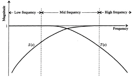
Figure 8.30 Representative sensitivity and complementary sensitivity frequency responses.
This results in a problem to the control-system engineer because we want the transfer function C(s)/N(s) to be as small as possible, but the desirable T(s) is large at low and mid-range frequencies as illustrated in Figure 8.30. Equation (8.217) showed that we would want to make T(s) = 1 ideally in order to drive the sensitivity function S(s) = 0. Therefore, the control-system engineer must make a tradeoff here between allowable feedback sensor measurement noise and the complementary sensitivity function (which also affects the sensitivity function [see Eq. (8.217)]. The basic tradeoff is to determine allowable noise and permissible sensitivity.
B. Desirable Control-System Transfer-Function Characteristics
From Figure 8.29 and Eq. (8.211), we can state the relationship between the reference input R(s), the disturbance U(s), and the feedback sensor measurement noise N(s) with the output C(s) as follows:
where
In terms of the error function E(s), as defined in Eq. (8.212), we define E(s) as follows:
It is interesting to examine the effect of the feedback sensor noise on the control system. To do this, let us assume that all the other external inputs are zero:
Let us assume that n(t) has a Fourier transform although, in practice, noise usually does not have a Fourier transform. Using Parseval’s theorem, we can determine the integral-squared error (ISE) which was defined in Chapter 5 by Eq. (5.45):
By focusing on the square of the error, the ISE penalizes both positive and negative values of the error. The function |N(jω)|2 is defined as the energy density spectrum of ω.
Let us try to define the desirable frequency characteristics from a practical viewpoint for Hr(jω), Hu(jω), and Hn(jω). The reference input R(s) and the disturbance U(s) are usually low-frequency signals. Therefore, it is desired to have Hr(jω) ≈ 1 and Hu(jω) ≈ 0 at low frequencies. In practice, Hr(jω) ≈ 0 and Hu(jω) and Hn(jω) ≈ 1 at high frequencies. In practice, we try to make Hr(jω) ≈ 1, and Hu(jω) and Hn(jω) ≈ 0 over the frequency range from 0 to the gain crossover frequency ωc. These are ideals and, in practice, we can only approximate these. For example, Figure 6.51b shows the closed-loop frequency response of Figure 6.51a. This closed-loop frequency response corresponds to Hr(s) for the system shown in Figure 6.51a.
In practice, G(s) is much greater than one at low frequencies. Therefore, Eq. (8.223) reduces to
and Eqs. (8.224) and (8.225) reduce to
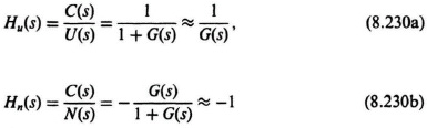
at low frequencies. Therefore, a high loop gain is very desirable for frequencies in the passband (defined as frequencies between 0 and ωc) because it then approximates Hr(jω) ≈ 1 and Hu(jω) is very small. However, the sensor measurement observation noise remains a problem because Hn(s) is approximately −1. The control engineer has two choices regarding N(s): (a) Design the sensor so that its measurement noise is very small; (b) tradeoff how high the loop gain is designed so that it minimizes the effect of the disturbance input U(s), but the loop gain should not be too high so that the effect of the noise is tolerable.
C. Extension of Sensitivity and Complementary Sensitivity Concepts to Multivariable Control Systems
Many modern control systems contain several inputs and outputs. Therefore, it is important to extend our understanding of sensitivity and complementary sensitivity to multiple-input multiple-output (MIMO) control systems.
Figure 8.31 illustrates the block diagram of a MIMO control system where r(t0) and c(t) are vectors, and D(s) and G(s) are matrices. The dimensions of D(s) are n × i, and the dimensions of G(s) are i × n, where n = dim[C(s)] and i = dim[m(s)]. By analogy to Eq. (8.213) for the SISO control system, the sensitivity function for the MIMO control system is given by:
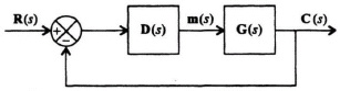
Figure 8.31 Block diagram of a MIMO control system.
By analogy to Eq. (8.216) for the SISO control system, the complementary sensitivity function for the MIMO control system is given by
The sensitivity and complementary sensitivity functions are both n × n matrices. By analogy to Eq. (8.217) for the SISO case, the sum of the sensitivity and complementary functions for the MIMO case is given by
where I represents the identity matrix.
D. Example for Finding S(s) and T(s) for a MIMO Control System
The open-loop transfer function matrix for a two-input, two-output control system to be analyzed is given by
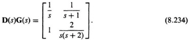
Let us determine the sensitivity and the complementary sensitivity functions.
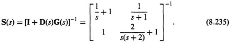
The sensitivity function for this MIMO control system is obtained from Eq. (8.231) as follows:
Therefore,
The complementary sensitivity function T(s) can be found from
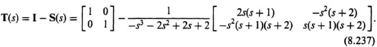
Simplifying this expression, we obtain