8.12.  FOUNDATIONS OF H^∞ CONTROL THEORY

Based on the preceding results, the concepts of modern H^∞ control theory will be presented. The very basic problem that H^∞ as presented by Zames in Reference 16 focuses on is sensitivity reduction of feedback control systems as an optimization problem, and it is separated from the problem of stabilization. The technique is concerned with the effects of feedback on uncertainty, where the uncertainty may be in the form of an additive disturbance U(s) as illustrated in Figure 8.29. H^∞ control theory approaches the problem from the point of view of classical sensitivity theory, which has been presented in Chapter 5 and subsections 8.11A–8.11D, with the difference that feedback will not only reduce but also optimize sensitivity in an appropriate sense.

H_∞ control theory is a complex subject. The purpose of presenting it in this book, which is designed for the undergraduate student and the practicing engineer, is to introduce it and motivate the reader with an interest in this field to review some of the recent research papers which have been written on this subject [18–20]. In its basic form, H^∞ control theory attempts to minimize the supremum function over the entire frequency range

where S(jω) is the sensitivity function and W(jω) is a weighting function. We can view the magnitude of the product S(jω)W(jω) as the magnitude of the weighted sensitivity. The weighting function emphasizes that low sensitivity is more important at low frequencies than higher frequencies. Therefore, by emphasizing the minimization of the magnitude of the product, the result is that the weighting function is greatest at those frequencies where the sensitivity is the smallest—namely at low frequencies.

The general solution to Eq. (8.239), obtained from function analysis, has the following general form [21]:

where k is a constant and B(s) is known as the Blaschke product. For the problem being considered in this book where the process G(s) is stable (e.g., all of its poles are in the left-half of the s-plane and are of minimum phase), then B(s) = 1 and the constant k is any desirable, small, real number. Therefore, Eq. (8.240) states that we want to make the weighting function large for those low frequencies where we want to make the sensitivity small. Conversely, we want to make the weighting function small for those high frequencies where the sensitivity is large.

Let us examine in detail the result when G(s) has all its poles in the left-half of the s-plane, and B(s) = 1. Therefore,

which implies that the shape of the magnitude of the sensitivity curve is the inverse of the weighting function. Therefore, the shape of the optimum |S(jω)| is independent of the process G(s), and only depends on the magnitudes of the constant k and the weighting function W(jω).

A.  Application of the Theory to an Example

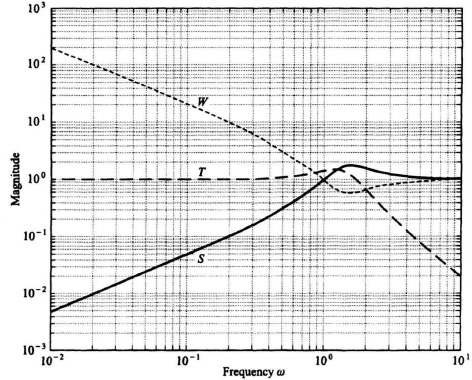
Let us try to pull all the concepts presented in this section together by giving an example. We will consider a simple SISO control system, and determine its sensitivity function, s, complementary sensitivity function, T, and the weighting function, W. We will also assume that the constant k in Eq. (8.240) is equal to one.

For the illustrative example, let us consider a unity-feedback control system whose forward transfer function G(s) is given by

Substituting Eq. (8.242) into Eqs. (8.213), (8.216), and (8.241), we can calculate the sensitivity S, the complementary sensitivity T, and the weighting function W, respectively. The result is shown in Figure 8.32. The result agrees with the theoretical results expected from the presentation of this section. The sensitivity S is very small at low frequencies, and approaches one at very high frequencies. The weighting function W is the inverse of the sensitivity function, and is very large at low frequencies and also approaches one at very high frequencies. The complementary sensitivity function equals one minus the sensitivity function (see Eq. (8.217)), and equals one at very low frequencies and is very small at very high frequencies.

B.  The H^∞ Process for the General SISO Case

Let us assume that in the general SISO case, the proces G(s) has poles in the right half-plane. For this general case, the H^∞ process would proceed in the following step-by-step manner:

1. The weighting function W(s) would be selected which would have the following characteristics:

• It must have no zeros in the right half-plane.

  

  Figure 8.32  S, T and W for a unity-feedback system with G(s) = 2/s(s + 1).

• It must contain any poles that G(s) has on the jω axis.
• It must not contain jω poles at zeros of G(s).

2. Determine the Blaschke product B(s) from knowledge of the poles of G(s). If G(s) has no poles in the right half-plane as illustrated in the preceding example in subsection 8.11A, B(s) = 1. Let us next consider the general case where G(s) has poles in the right half-plane. Therefore, from Eq. (8.240),

where p_n are poles of G(s) in the right half-plane.

3. S(p_n) has to satisfy the following interpolation conditions for simple poles and zeros of G(s) in the right half-plane:

• S equals zero at right-half poles, and one at right-half zeros.
• T is one at right-half poles and zero at right-half zeros.

This can be shown as follows. Let us consider the control system in Figure 8.33. The sensitivity of C(s)/R(s) to D(s)G(s) is given by

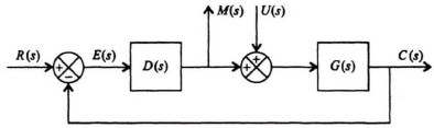
Figure 8.33  General SISO control system containing a reference input, R(s), and a disturbance signal, U(s).

The complementary sensitivity function is given by

The transfer functions between the inputs R(s) and U(s), and the outputs M(s) and C(s) are given as follows:

In terms of T(s) given by Eq. (8.245), Eq. (8.246) can be written as

Therefore,

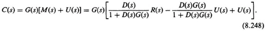
Equation (8.248) can be reduced to the following:

In terms of T(s) and S(s), Eq. (8.249) can be rewritten as follows:

Analysis of Eq. (8.247) reveals the following:

• If T(s)/G(s) is to be stable, then T(s) must cancel the right-half zero(s) of G(s).

Analysis of Eq. (8.250) reveals the following:

• If G(s)S(s) is to be stable, then S(s) must cancel the pole(s) in the right-half plane of G(s).

These two very important interpolation conditions imply that for simple zeros and poles which are in the right half-plane, S(s) equals one at the right-half-plane zeros, and S(s) equals zero at the right-half-plane zeros, and S(s) equals zero at the right-half plane poles. Similarly, T(s) equals zero at the right-half-plane zeros, and T(s) equals one at the right-half-plane poles.

4. Form the Blaschke product. Returning to Eq. (8.243), and recognizing that S(p_n) must satisfy these interpolation conditions, what should B(p_n) and W(p_n) be? Let us assume that G(s) has poles in the right half of the s-plane, and let P_n, n = 1, 2, ... , N, be poles of G(s). Therefore, Eq. (8.243) must be satisfied for the interpolation conditions. Because the weighting function W(s) has no poles in the right half-plane, it cannot equal infinity. Therefore, it is necessary to have the Blaschke product B(s) contain the zeros of S(p_n): B(p_n) = 0, n = 1, 2, 3 ..., N. This means that the Blaschke product accounts for these zeros as follows:

where

We can find B′(s) from the interpolation conditions previously shown. For example, let us assume that these zeros in the right half-plane which force S(s) to equal one at these zeros are z₁, z₂, z₃, ... , z_M. From Eqs. (8.243) and (8.251),

This equation can be simplified to

Equation (8.254) represents M equations which must be solved. It can be shown that if M = 1, then B′(s) = 1. If M is greater than one, then

where c_i are complex values with the positive real parts chosen, together with the value of k, to satisfy Eq. (8.254).

5. Solve for S(s). Having solved B′(s), the optimal sensitivity S(s) is then calculated from the following equation which is obtained by substituting Eq. (8.251) into Eq. (8.240):

The resulting S(s) is stable because B′(s) and B_p(s) are stable, and since W(s) has no poles in the right half-plane. Because |B(jω)| = 1

Therefore, this equation shows that the magnitude of the sensitivity curve is the inverse of the magnitude of the weighting function curve. It is also interesting to observe that the optimal |S(jω)| is independent explicitly of G(s). However, G(s) does effect the value of k.

C.  An Example of the SISO Case Containing a Pole in the Right Half-Plane

Consider the control system illustrated in Figure 8.33 where

and the weighting function W(s), shown in Figure 8.34, is given by

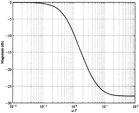
Figure 8.34  Weighting function W(s).

This weighting function gives more weight to low frequencies (up to the bandwidth 1/2T) than high frequencies. From Eq. (8.252), the right-half pole of G(s) at s = 3 results in B_p(s) given by

Because D(s)G(s) has only one zero at s = 2 in the right half-plane of the s-plane, then B′(s) = 1. Therefore, from Eq. (8.254), we can find k as follows:

Substituting k from Eq. (8.261), B_p(s) from Eq. (8.260), and W(s) from Eq. (8.259) into Eq. (8.256) we can solve for the optimal sensitivity S(s):

We can obtain the absolute value of the optimal sensitivity function from Eq. (8.257) as follows:

Figure 8.35 illustrates the absolute value of the sensitivity function obtained from Eq. (8.263) for values of T = 0.2, 2, and 20. It is concluded from this curve that the sensitivity is smaller (better) at low frequencies if the bandwidth is not too high (or T is not too small).