
6.23. ILLUSTRATIVE PROBLEMS AND SOLUTIONS
This section provides a set of illustrative problems and their solutions to supplement the material presented in Chapter 6.
A control system can be represented by the following companion matrix:

(a) Determine the characteristic equation.
(b) Determine the location of the route of the characteristic equation.
(c) Is the control system operating in a stable region?
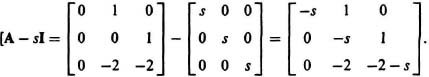
Using minors along the first column, we obtain the following:
![]()
Therefore, the characteristic equation is given by the following:
s(s2 + 2s + 2) = 0
(b) Since
s(s2 + 2s + 2) = s(s + 1 + j)(s + 1 − j) = 0
the roots of the characteristic equation are given by the following:
s1 = 0,
s2 = −1 − j,
s3 − 1 + j.
(c) Because the complex-conjugate roots have negative real parts, and the third root is located at the origin, none of the roots are located in the right half-plane and the system is operating in a stable region.
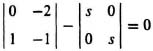
I6.2. A second-order control system can be represented by the following companion matrix:
![]()
(a) Determine the characteristic equation of this control system.
(b) Determine the location of the roots of the characteristic equation.
(c) Is this control system operating in a stable region?
SOLUTION: (a) From Eq. (6.21):
|P − sI| = 0
or,
![]()
Therefore, the characteristic equation is given by:
s2 + s + 2 = 0.
(b)
s2 + s + 2 = (s + 0.5 + 1.325j)(s + 0.5 − 1.325j),
s1 = −0.5 − 1.325j,
s2 = −0.5 + 1.325j.
(c) Since the complex-conjugate roots are located in the left half-plane, the system is stable.
I6.3. A control system containing a tachometer, which provides rate feedback, is illustrated. Determine the range of the tachometer constant, b. in order that the system is always stable.

Figure I6.3
SOLUTION: Using Mason’s Theorem, we obtain:

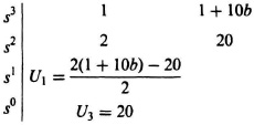
Setting U1 = 0, we obtain:
![]()
Therefore, b = 0.9, and the tachometer constant, b, must be
b > 0.9
for the system to be stable.
I6.4 The forward-loop transfer function of a unity-feedback control system is given by the following:
![]()
Determine the values of K and T for stability of this control system.
SOLUTION:
![]()
The characteristic equation is given by
Ts3 + (4T + 1)s2 +(4 + K)s + K = 0.
The Routh–Hurwitz array is given by:
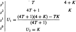
Analysis of this Routh–Hurwitz array, shows that the system will be stable if K and T are both greater than zero.
I6.5. The forward-loop transfer function of a unity-feedback control system is given by the following:
![]()
(a) Sketch the Nyquist diagram, and determine whether the control system is stable.
(b) Determine the intersection of the G(jω)H(jω) and the negative real axis of the G(jω)H(jω) plane analytically, and find the values of the frequency, ω, and location of the intersection on the negative real axis.
(c) How much can the system gain, 2, be increased before the roots of the characteristic equation cross the jω axis and go into the right-half plane?
SOLUTION: (a)
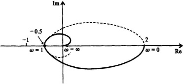
Figure I6.5 Solution.
(b)
![]()
Separating the real and imaginary terms in the denominator, we obtain the following:
![]()
Therefore,
![]()
Setting the imaginary part of the numerator equal to zero, we obtain:
−2(4ω − 4ω3) − 0.
Therefore,
ω = 0, 1 −1
and we are interested in the condition ω = 1. The case of ω = 0 refers to the intersection of the Nyquist diagram with the positive real axis.
Substituting ω = 1 into G(jω), we obtain that the intersection of the Nyquist diagram and the real axis occurs at −0.5.
(c) Since the intersection of the Nyquist diagram and the negative real axis occurs at −0.5, we can increase the gain, 2, to 4 at which point the Nyquist diagram crosses the negative real axis at −1 and the roots of the characteristic equation cross the jω axis.
I6.6. The open-loop transfer function of a feedback control system is given by the following:
![]()
(a) Sketch the Nyquist diagram, and determine whether the control system is stable.
(b) Determine the intersection of the G(jω)H(jω) and the negative real axis of the G(jω)H(jω) plane analytically, and find the values of the frequency, ω, and location of the intersection on the negative real axis.
(c) What is the maximum value of gain for this control system before the roots of the characteristic equation cross the jω axis and go into the right half-plane?
SOLUTION: (a)

Figure I6.6 Solution.
N = Z − P
Since P = 0, and N = +2, Z = 2, there are two roots in the right half-plane and the system is unstable.
![]()
Therefore,
![]()
Setting the imaginary part of the numerator equal to zero, we obtain:
20j(ω − 0.08ω3) = 0
ω2 = 12.5.
Therefore,
ω = 3.536 rad/sec and − 3.536 rad/sec.
So, G(jω)H(jω) intersects the negative real axis at ω = 3.536 rad/sec. Substituting this value of ω into the equation for G(jω)H(jω), we find that the intersection of G(jω)H(jω) with the negative real axis occurs at:
G(j3.536)H(j3.536) = −2.6667.
(c) Therefore, the value of gain for the G(jω)H(jω) plane to cross the negative real axis at −1 is given by
![]()
Thus, the maximum value of gain for this control system before the roots of the characteristic equation cross the jω axis and go into the right half-plane is 7.5.
I6.7. An engineer is called in to consult on a control system in a piece of equipment in the field. No one can find the design report or test results from the original design of the control system. The engineer, therefore, decides to take a frequency response of the control system by opening the outer feedback loop. The resulting asymptotic gain-frequency characteristic is obtained:
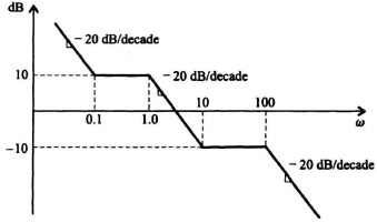
Figure I6.7 Asymptotic gain frequency characteristic solution
Assuming that the system has a minimum phase transfer function, determine the transfer function, G(s)H(s).
SOLUTION: From knowledge of the break points, we know that the transfer function is given by the following transfer function where K is the gain to be determined:
The value of K can be obtained from knowledge that at ω = 0.1 rad/sec, the gain is 10 dB. Therefore,
![]()
Therefore, K = 0.316 and the complete transfer function is given by:
![]()
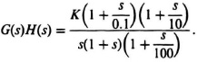
I6.8. (a) Determine the root locus for a unity-feedback control system whose forward transfer function is given by
![]()
(b) Determine the location of the roots when all three roots are all real and equal.
(c) Find the gain when all the roots are real and equal.
SOLUTION: (a) See root locus plot (Figure I6.8) using MATLAB.
Figure I6.8 Root-locus plot solution.
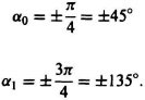
The angles of the intersection of the asymptotes and the real axis are given by:
![]()
The intersection of the asymptotes and the real axis is given by:
![]()
(b) We can find the location of the roots when they are all equal from Rule 7 as follows:
![]()
Solving for K, we obtain the following:
![]()
Limiting s to the real axis, we let s = σ Therefore,
Taking the derivative of K(σ) with respect to σ we obtain:
![]()
Simplifying this equation, we obtain the following:
2σ(σ2 + 12σ + 36) = 0.
Solving, we find that σ = 0 and −6. Therefore, at σ = −6 all three roots intersect and are real. We can find the value of gain when all the roots are equal at σ = −6 by substituting σ = −6 into Eq. (I6.8-1). Therefore, we find that K = 108.
(a) Draw the root locus of a negative feedback, unity-feedback control system whose forward-path transfer function is given by the following:
![]()
(b) At what value of K does the system become unstable, and where does the root locus intersect the jω axis when this occurs?
SOLUTION: (a)
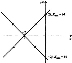
Figure I6.9 Root-locus plot solution
Rule 5: Asymptotes are given by
Rule 6: Intersection of the asymptotes and the real axis is given by:
![]()
(b) Rule 8: The intersection of the root locus and the imaginary axis and Kmax are found from this rule. The characteristic equation is given by:
![]()
which simplifies to the following:
s4 + 8s3 + 24s2 + 32s + 16 + K = 0.
The intersection of the root locus and the imaginary axis can be determined by substituting s = jω into the characteristic equation:
(jω)4 + 8(jω)3 + 24(jω)2 + 32jω + 16 + K = 0.
Setting the imaginary terms equal to zero, we obtain:
−8(jω)3 + 32jω = 0
jω[−8ω2 + 32] = 0.
Therefore, ω = ±2, and the root locus crosses the imaginary axis at ±2j.
The value of Kmax can be determined from the following Routh–Hurwitz array:

Setting the term in the fourth row equal to zero, we obtain
![]()
Therefore, Kmax = 64.
I6.10. Consider a negative-feedback control system whose open-loop transfer function is given by:
![]()
(a) Sketch the root locus.
(b) Determine when the roots are both equal.
(c) Determine the gain when these two roots are both equal.
(d) Determine the settling time when the roots are equal.
SOLUTION: (a)
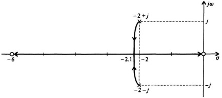
Figure I6.10 Root-locus plot solution.
(b) Rule 7: To find the point of breakaway, we start with the characteristic equation:
![]()
We restrict s to real values, let s = σ, and we solve for K:
![]()
Taking the derivative of K(σ) with respect to σ, we get the following:
![]()
Simplifying, we obtain the following:
![]()
Therefore:
σ2 − 5σ − 15 = 0.
Therefore, the two resulting roots of this equation are:
σ1 = −2.1,
σ2 = 9.1.
Only σ1 is a valid solution for negative feedback. Therefore, the roots are both equal at σ1 = −2.1.
(c) The gain when the two roots are equal can be determined from Rule 11:
![]()
Therefore, K = 0.134.
(d) We can determine the settling time from Eq. (5.41):
![]()
In this equation, the damping ratio ζ equals one because the two roots are on the real axis, and ωn equals the intersection value on the real axis. Therefore,
![]()
Therefore, the settling time is 1.9 sec when the roots are equal.