6.2.  DETERMINING THE CHARACTERISTIC EQUATION USING CONVENTIONAL AND STATE-VARIABLE METHODS

The characteristic equation can be defined in terms of the state-variable equation of the control system. We have stated in the previous section that stability of linear systems is independent of the input. Therefore, the condition x(t) = 0, where x(t) is the state vector, can be viewed as the equilibrium state of the system. Let us assume that a linear system is subjected to a disturbance at t = 0, resulting in an initial state x(0) that is finite. If it returns to its equilibrium state as t approaches infinity, the system is considered to be stable. If it does not, in terms of our definition, it is considered to be unstable. These concepts of stability can be generalized. In the state-variable approach [1, 2], a linear system is considered to be stable if, for a finite initial state x(0), there is a positive number A that depends on x(0), where

The value x(t) denotes the norm of the state vector x(t). It is defined as

Equation (6.8) can be interpreted to mean that the transition of state for positive time, as represented by the norm of the vector x(t), is bounded. Equation (6.9) can be interpreted to mean that the system must reach its equilibrium point as t approaches infinity. Figure 6.3 shows the state-variable stability criterion for a second-order system having states x₁(t) and x₂(t). Observe from this figure that a cylinder, the radius of which is A, forms the bound for the trajectory as time increases. As time approaches infinity, the linear system reaches the equilibrium point x(t) = 0. Note that, strictly speaking, the above definition corresponds to asymptotic stability.* For simplicity, we will call the system stable if Eqs. (6.8) and (6.9) hold.

Let us next develop analytically, and apply, the state-variable approach for determining the stability of a linear system. It will be shown that this method determines the location of the roots of the characteristic equation, and restricts the roots of the characteristic equation to the left half-plane for stability.

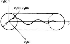
Figure 6.3   State-space stability concept.

Consider the general differential equation of a linear system in scalar form:

where all the coefficients are constants, A_n ≠ 0, r(t) represents the input to the system, and c(t) represents the system output. The Laplace transform of Eq. (6.11) is given by

Stability can be determined from the characteristic equation of this system:

It remains now to determine the roots of this equation.

The nth-order differential equation, given by Eq. (6.11), may also be specified by n first-order differential equations. By defining

the linear system can be specified by the following set of first-order differential equations:

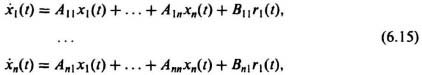
which is equivalent to Eq. (6.11).

The set of equations (6.15) is solved for the case where the input r(t) equals zero; assume an exponential solution of the form

where f_i is an unknown constant. To check the form of the assumed solution, Eq. (6.16) is differentiated and the result is substituted into the set of equations (6.15). Differentiating (6.16), we obtain

Substitution of Eqs. (6.16) and (6.17) into (6.15) results in

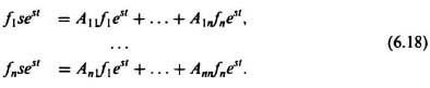
Equating coefficients of e^st and rearranging, we obtain the following:

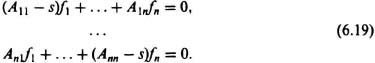
This set of equations can be rewritten in the following matrix algebra form:

where f = column matrix, or vector, and I = identity matrix. Observe that matrix A used in Eq. (6.20) is analogous to the P matrix introduced in Chapter 2 when state variables were introduced [see Eq. (2.197]. Equation (6.20) will have a nontrivial solution only if

By expanding the determinant |A − sI| and solving for the roots of the equation |A − sI| = 0, eigenvalues of matrix A are obtained. Expanding the determinant

results in the following expression:

Notice that the B_i terms in Eq. (6.23) are equivalent to the A_i/A_n terms in Eq. (6.13). Therefore, the two equations are equivalent. The n values of s that satisfy Eq. (6.22) are called the characteristic values, or eigenvalues, of the matrix.

As an example for comparing the stability determination of a system utilizing conventional Laplace-transform and state-variable techniques, consider the unity-feedback system shown in Figure 6.4. Using the Laplace transform, we could easily obtain the closed-loop transfer function of the system as

The characteristic equation of this simple linear system is given by

System stability can be determined by locating the roots of this equation if the classical approach is to be used. The same problem will next be analyzed from the state-variable viewpoint.

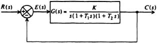
Figure 6.4   Third-order feedback control system.

From Eq. (6.24), we obtain

The time-domain expression equivalent to Eq. (6.26) is given by

As discussed previously, this third-order differential equation may be written as three first-order differential equations as follows:

This can easily be transformed into matrix form:

Using vector and matrix notation, the above equation becomes

where

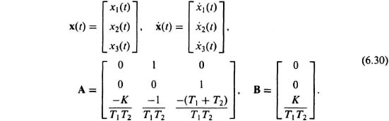
In order to obtain the characteristic equation, the input will be set equal to zero and the solution x_i will be assumed equal to f_ie^st. As outlined previously [see Eq. (6.22)], this procedure results in

The resulting determinant is given by

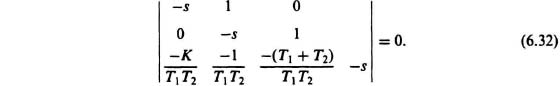
Expansion of the determinant by means of minors along the first row gives

which reduces to

Equation (6.34), obtained utilizing the state-variable approach, is the same characteristic equation as (6.25), which was obtained by using conventional Laplace-transform techniques. Although the mathematics involved in obtaining Eq. (6.34) was more laborious than for Eq. (6.25) for this simple problem, many important features and characteristics of the state-variable approach have been presented and applied. It is important to emphasize that for more complex problems involving multiple inputs and outputs, the state-variable approach greatly simplifies the solution. In addition, it greatly facilitates computation utilizing digital computers.