2.15  REDUCTION OF THE SIGNAL-FLOW GRAPH

Several preliminary simplifications can be made to the complex signal-flow graphs of a system by means of the following signal-flow graph algebra.

(a)  Addition

1. The signal-flow graph in Figure 2.13a represents the linear equation

2. The signal-flow graph in Figure 2.13b represents the linear equation

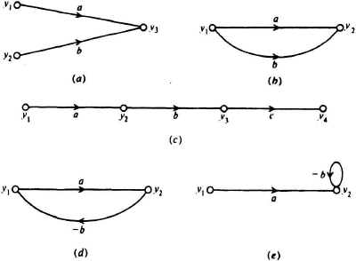
Figure 2.13   Signal-flow graph algebra.

(b)  Multiplication. The signal-flow graph in Figure 2.13c represents the linear equation

(c)  Feedback loops

1. The signal-flow graph in Figure 2.13d represents the linear equation

2. The signal-flow graph in Figure 2.13e represents the linear equation

It is possible to apply the preceding signal-flow graph algebra to a complicated graph and reduce it to one containing only a source and a sink. This process requires repeated applications until the final desired form is obtainable. An interesting property of network and system topology, based on Mason’s theorem [7, 8] permits the writing of the desired answer almost by inspection. The general expression for signal-flow graph gain G is given by

where

Δ = 1 − ΣL₁ + ΣL₂ − ΣL₃ + ... + (−1)^m ΣL_m

L₁ = gain of each closed loop in the graph

L₂ = product of the loop gains of any two nontouching closed loops (loops are considered nontouching if they have no node in common)

        . . . . . . . . . . . . . . . . . . .

L_m = product of the loop gains of any m nontouching loops

G_K = gain of the Kth forward path

Δ_K = the value of Δ for that part of the graph not touching the Kth forward path (value of Δ remaining when the path producing G_K is removed).

Δ is known as the determinant of the graph and Δ_K is the cofactor of the forward path K. Basically, Δ consists of the sum of the products of loop gains taken none at a time (1), one at a time (with a minus sign), two at a time (with a plus sign), etc.; Δ_K contains the portion of Δ remaining when the path producing G_K is removed. The proof of this general gain expression is contained in Reference [8]. A few examples follow in order to show how this expression may be used.

Example 1. For Figure 2.14a,

       Δ = 1 − bd,

 G₁ = abc,

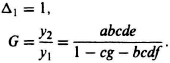
Δ₁ = 1.

Therefore,

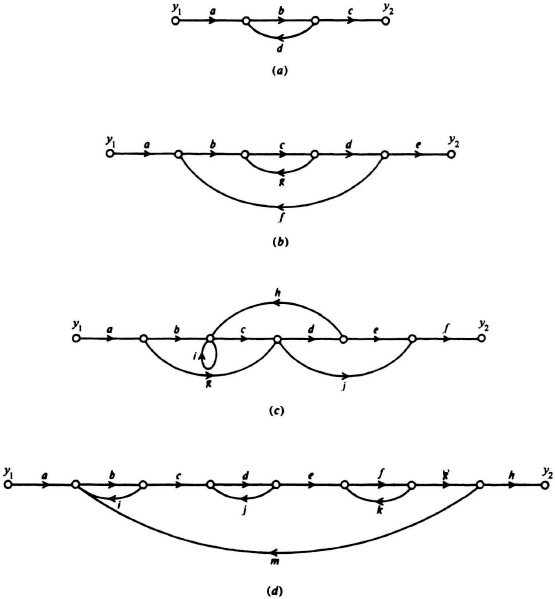
Figure 2.14   Signal-flow graph examples: (a) Example 1, (b) Example 2, (c) Example 3, (d) Example 4.

Example 2. For Figure 2.14b,

           Δ = 1 − cg − bcdf

G₁ = abcde.

Therefore,

Example 3. For Figure 2.14c,

          Δ = 1 – (i + cdh),

G₁ = abcdef,

G₂ = agdef,

G₃ = agjf,

G₄ = abcjf,

                       Δ₁ = 1,             Δ₃ = 1 – i,

                   Δ₂ = 1 – i,        Δ₄ = 1.

Therefore,

Example 4. For Figure 2.14d,

  Δ = 1 − (bi + dj + fk + bcdefgm) + (bidj + bifk + djfk) – bidjfk,

G₁ = abcdefgh,

Δ₁ = 1.

Therefore,