2.20.  REVIEW OF MATRIX ALGEBRA

The classical methods of describing a linear system by means of transfer functions, block diagrams, and signal-flow graphs have thus far been presented in this chapter. An inherent characteristic of this type of representation is that the system dynamics are described by definable input-output relationships. Disadvantages of these techniques, however, are that the initial conditions have been neglected and intermediate variables lost. The method cannot be used for nonlinear, or time-varying systems. Furthermore, working in the frequency domain is not convenient for applying modern optimal control theory, discussed in Chapter 6 of the accompanying volume, which is based on the time domain. The use of digital computers also serves to focus on time-domain methods. Therefore, a different set of tools for describing the system in the time domain is needed and is provided by state-variable methods. As a necessary preliminary, matrix algebra is reviewed in this section [5, 10].

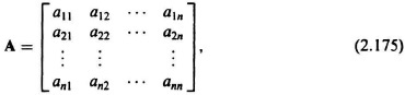
A matrix A is a collection of elements arranged in a rectangular or square array defined by

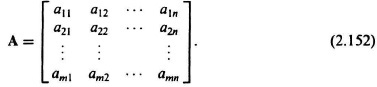
The order of a matrix is defined as the total number of rows and columns of the matrix. For example, a matrix having m rows and n columns is referred to as an m × n matrix. A square matrix is one for which m = n. A column matrix, or vector, is one for which n = 1, and is represented in the following manner:

A row matrix or row vector is one that has one row and more than one column (e.g., a 1 × n matrix). Capital letters are used to denote matrices and lower-case letters to denote vectors. Matrix A equals matrix B if element a_ij equals element b_ij for each i and each j, where the subscripts refer to elements in row i and column j of the respective matrices.

Before the basic types of properties of matrices are presented, let us note the differences between a matrix and a determinant. First, a matrix is an array of numbers or elements having m rows and n columns, while a determinant is an array of numbers or elements with m rows and n columns and is always square (m = n). The second major difference is that a matrix does not have a value while a determinant has a value. In addition, note that a square matrix (m = n) has a determinant. A matrix is said to be singular if the value of its determinant is zero.

In order to present the basic types and properties of matrices, matrix A will be considered in the following discussion where the representative element is a_ij.

A.  Identity Matrix

The identity matrix, or unit matrix, is a square matrix whose principal diagonal elements are unity, all other elements being zero. This matrix, which is denoted by I, is given by

An interesting property of the identity matrix is that multiplication of any matrix A by an identity matrix I results in the original matrix A:

where matrix multiplication is defined later on.

B.  Diagonal Matrix

A diagonal matrix, which is denoted by diag x_i, is given by

C.  Transpose of a Matrix

A matrix is transposed by interchanging its rows and columns. To form the transpose of a matrix, element a_ij, which is the element of row i and column j, is interchanged with element a_ji, which is the element of row j and column i, for all i and j. For example, the transpose A, where

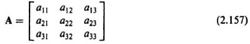
is written as A^T, where

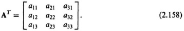
Note that the transpose of A^T is (A^T)^T = A.

D.  Symmetric Matrix

A symmetric matrix is defined by the condition

This matrix, which is denoted by A_s, is represented by

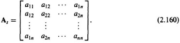
Notice that it is symmetrical about the principal diagonal, and that a symmetric matrix and its transpose are identical.

E.  Skew-Symmetric Matrix

A skew-symmetric matrix is defined by the condition

This matrix, which is denoted by A_a, is represented by

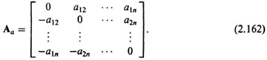
Note that a skew-symmetric matrix is equal to the negative of its transpose.

F.  Zero Matrix

The zero matrix or null matrix, denoted by 0, is defined as the matrix whose elements are all zero. It has the property that

where addition of matrices is defined later on.

G.  Adjoint Matrix

The adjoint of a square matrix is formed by replacing each element of the matrix by its corresponding cofactor, and then transposing the result. For example, if a matrix A is given by

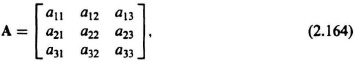
then the cofactors of the elements a₁₁, a₂₁ are given, respectively, by the determinants

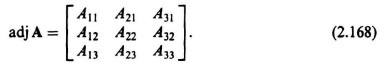
The element a_ij has for its cofactor A_ij with the proper algebraic sign, (−1)^i+j, prefixed. The new matrix formed by replacing the original elements in the matrix with their corresponding cofactors is given by

The transpose of this matrix results in the expression for the adjoint (adj) of matrix A:

In order to present the basic operations of matrix analysis, three matrices A, B, and C will be considered in the following discussion where the representative elements are denoted by a_ij, b_ij, c_ij.

H.  Addition or Subtraction

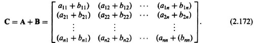
The sum (or difference) of two matrices A and B with the same numbers of rows and columns is obtained by adding (or subtracting) corresponding elements. The result is a new matrix C, where

and

For example, if matrices A and B are given by

then the sum of matrix A and matrix B is given by

I.  Multiplication of a Matrix by a Scalar

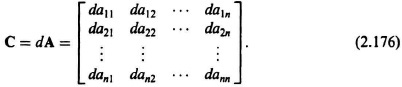
Multiplication of a matrix A by a scalar d is equivalent to multiplying each element of the matrix by d. The result is a new matrix C, where

and

For example, if matrix A is given by

then the multiplication of matrix A by scalar d is given by

J.  Multiplication of Two Matrices

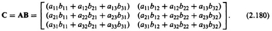
Postmultiplication* of matrix A by matrix B results in a new matrix C, where

and

These equations state that the result of postmultiplication of matrix A by matrix B is a matrix C whose element located in row i and column j is obtained by multiplying each element in row i of matrix A by the corresponding element in column j of matrix B and then adding the results. It is important to note that the number of columns in matrix A must equal the number of rows in matrix B so that matrices A and B may be multiplied together. For example, if matrices A and B are given by

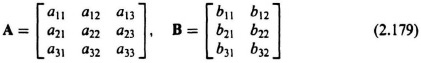
then the product of matrices A and B is given by

Matrix multiplication is associative and distributive with respect to addition, but in general not commutative:

K.  Inverse of a Square Matrix

The inverse of a square matrix B is denoted by B⁻¹ and has the property

It can be shown that the product of an adjoint matrix with the matrix itself has the property that it is equal to the product of an indentity matrix and the determinant of the matrix:

Using these two relationships, we can derive the expression for the inverse matrix B⁻¹. By solving for I from Eq. (2.185), the following relationship is obtained:

Using Eqs. (2.184) and (2.186), we obtain

Solving for the inverse matrix B⁻¹ in terms of the adjoint matrix and the determinant of the matrix, we obtain the following expression:

or

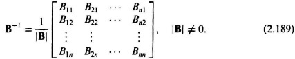
Note that B⁻¹ does not exist if |B| = 0, although Eq. (2.185) still holds.

L.  Differentiation of a Matrix

The usual concepts regarding the differentiation of scalar variables carry over to the differentiation of a matrix. Let A be an m × n matrix whose elements a_ij(t) are differentiable functions of the scalar variable t. The derivative of A with respect to the variable t is given by

In addition, the derivative of the sum of two matrices is the sum of the derivatives of the matrices:

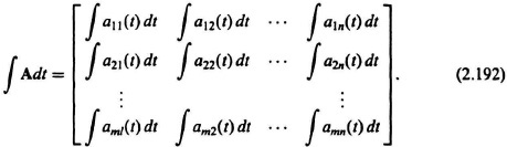
M.  Integration of a Matrix

The usual concepts regarding the integration of scalar variables also carry over to the integration of a matrix. Again, let A be an m × n matrix whose elements a_ij(t) are integrable functions of the scalar variable t. The integration of A with respect to the variable t is given by