2.6.  IMPORTANT PROPERTIES OF THE LAPLACE TRANSFORM

The Laplace transform has been introduced in order to simplify several mathematical operations. These operations center upon the solution of linear differential equations. Several basic properties of the Laplace transform are given here.

A.  Addition and Subtraction

If the Laplace transforms of f₁(t) and f₂(t) are F₁(s) and F₂(s), respectively, then

[f₁(t) ± f₂(t)] = F₁(s) ± F₂(s).

B.  Multiplication by a Constant

If the Laplace transform of f(t) is F(s), the multiplication of the function f(t) by a constant K results in a Laplace transform KF(s).

C.  Direct Transforms of Derivatives

If the Laplace transform of f(t) is F(s), the transform of the first time derivative (t) of f(t) is given by

where f(0⁺) is the initial value of f(t), evaluated as t → 0 from the positive region. The transform of the second time derivative (t) of f(t) is given by

where (0⁺) is the first derivative of f(t) evaluated at t = 0⁺. The Laplace transform of the nth derivative of a function is given by

The notation f⁽ⁿ⁻¹⁾(0⁺) represents the (n − 1)th derivative of f(t) with respect to time evaluated at t = 0⁺.

D.  Direct Transforms of Integrals

If the Laplace transform of f(t) is F(s), the transform of the time integral of f(t) is given by

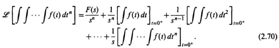
where [ f(t)dt]_t=0⁺ signifies that the integral is evaluated as t → 0 from the positive region. In general, for nth-order integration,

E.  Time-Shifting Theorem

The Laplace transform of a time function f(t) delayed in time by T equals the Laplace transform of f(t) multiplied by e^−sT:

F.  Frequency-Shifting Theorem

If the Laplace transform of f(t) is F(s), then the Laplace transform of

e^−atf(t)

is obtained as follows:

Therefore, multiplying f(t) by e^−at is equivalent to replacing s by (s + a) in the Laplace transform. In addition, changing s to (s + a) is equivalent to multiplying f(t) by e^−at.

G.  Initial-Value Theorem

If the Laplace transform of f(t) is F(s), and if lim_s→∞ sF(s) exists, then the initial value of the time function is given by

H.  Final-Value Theorem

If the Laplace transform of f(t) is F(s), and if sF(s) is analytic on the imaginary axis and in the right half-plane, then the final value of the time function is given by