8.7.  ESTIMATOR DESIGN IN CONJUNCTION WITH THE POLE PLACEMENT APPROACH USING LINEAR-STATE-VARIABLE FEEDBACK

In the discussion of Sections 8.2 and 8.3 on linear-state-variable feedback, it was assumed that all of the states are observable and measurable, and available to accept control signals (controllable). As Sections 8.4 and 8.5 on controllability and observability have shown, some states of a feedback control system may not always be controllable and/or observable. In some systems, the system may be observable, but all of the states may not be measured due to physical limitations (e.g., chemical process control systems), or it may be due to cost restrictions that limit the use of costly sensors needed to measure all of the states. It is assumed in this section that the system is observable (no part of the system is disconnected physically from the output), but measurements are being made only on some of the states, and we wish to estimate all of the states.

Let us focus attention on the process portion of the system illustrated in Figure 8.3. We wish to use the closed-loop estimator system shown in Figure 8.18 for determining an estimate of the state vector x(t) and output c(t) [8]. This estimator feeds back the difference between the measured output c(t) and the estimated output ĉ(t) that is obtained from a model of the process. Therefore,

where M defines the gain factors m_i, which are selected to obtain desirable error characteristics of the state vector x, and (t) represents the estimate of the state x(t):

The error in the state estimate, (t), can be derived from

Figure 8.18  An estimator system.

The derivative of the (t) can be obtained by subtracting (t) [given by Eq (8.120)] from (t) [given by the system dynamics:

Subtracting Eq (8.120) from Eq (8.123), we obtain the following:

Substituting Eq. (8.2),

into Eq. (8.126), we obtain

Using the definition of error in the state estimate as given by (8.122), Eq (8.128) reduces to

or

We have shown in Section 6.2 on the state-variable determination of the characteristic equation that a state equation, as given by Eq. (6.15),

has a characteristic equation given by Eq. (6.22). Similarly, the characteristic equation of Eq (8.129) is given by

The objective of the control-system engineer is to select P − ML so that it has stable roots in order for (t) to decay to zero. It is also desirable to have the root location produce a fast transient response so that the estimation error decays very fast to zero. Notice that the estimation error (t) will converge to zero independent of the forcing function u(t). Therefore, stability is determined from the homogeneous solution to the sysem (with u(t) = 0), as opposed to its particular solution (with u(t) finite).

The design procedure for determining M is to specify the desired location of the estimator roots (e.g., α₁ α₂,...,α_n) from which the desired estimator characteristic equation can be specified:

We can then solve for M by comparing the coefficients in Eqs (8.131) and (8.132).

Let us consider the design of M for a simple second-order system whose differential equation is given by

(t) + (t) + c(t) = u(t).

Defining its two states as

x₁(t) = c(t)
 x₂(t) = (t),

we obtain its state equations as

₁(t) = x₂(t)                         
₂(t) = −x₁(t) − x₂(t) + u(t),

and its output equation as

Therefore, for this system, we obtain P, b, and L to be as follows:

Substituting Eq (8.134) into Eq (8.131), we obtain the following:

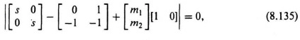
The resulting characteristic equation is given by

Where do we desire to place the two second-order roots? We could use the ITAE criterion, presented in Section 5.8, to make that determination. However, here the primary goal is to design the estimator to be very fast compared to that of the controller. Therefore, let us assume that the controller is critically damped and the controller’s second-order characteristic equation has a pair of real roots located at s = β₁ = β₂ = 2. Let us assume that we wish the estimator to be critically damped and have the two second-order roots of the estimator located at α₁ = α₂ = 20 in Eq (8.132), which will ensure a very fast response compared to that of the controller. Therefore, Eq (8.132) for this example becomes

Comparing the coefficients of Eqs. (8.138) and (8.139), we obtain the following two sumultaneous equations to solve:

Solving Eqs. (8.140) and (8.141), we obtain:

Designing a combined compensator of a controller and estimator is illustrated in Section 8.8.