
8.10. ROBUST CONTROL SYSTEMS [10–14]
Robust control is concerned with determining a stabilizing controller that achieves feedback performance in terms of stability and accuracy requirements, but the control must achieve the performance that is robust (insensitive) to plant uncertainty, parameter variation, and external disturbances. We know from the previous discussion in this book that feedback reduces the effects of external disturbances (Section 2.17) and parameter variations (Section 5.3). However, this is only achieved with relatively high loop gain which limits stability. Robust control is basically the same problem that was addressed in the 1930s by Black, Bode, and Nyquist. Modern robust control revolves around the feedback configurations illustrated in Figures 7.5, 7.6, and 7.7 which illustrate two-degrees-of-freedom compensation systems.
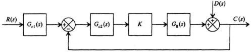
Figure 8.23 Control system with a two-degrees-of-freedom series controller Gc1(s) and a forward-loop-controller Gc2(s).
Let us consider the control system illustrated in Figure 8.23 which contains a disturbance D(s), and it contains a two-degrees-of-freedom series controller Gc1(s) and a forward-loop controller Gc2(s). In this control system’s operation, the amplifier gain, K, can vary.
For this control system, the overall transfer function, C(s)/R(s), is given by
The transfer function relating the disturbance D(s) to the output C(s) is given by
The design approach in robust control systems is to choose the controller Gc1(s) so that the desired closed-loop transfer function H(s) is obtained, and to choose the controller Gc2(s) so that the output, C(s), is insensitive to the disturbance D(s) over the frequency range in which D(s) is dominant.
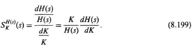
The sensitivity of H(s) due to variations of K is given by
For the control system of Figure 8.23,
Substituting Eqs. (8.197) and (8.200) into Eq. (8.199), we obtain the following:
It is important to recognize that for this control system, both C(s)/D(s) given by Eq. (8.198) and the sensitivity of H(s) with respect to K given by Eq. (8.201) are identical. This is a very important result which implies that we can use the same control-system techniques to suppress the affect of the disturbance D(s) and robustness (insensitivity) with respect to variations of K.
A. Design Example Illustrating Robustness and Disturbance Rejection
We will next analyze how the two-degrees-of-freedom control system illustrated in Figure 8.23 can achieve a high-gain which will satisfy the robustness and performance requirements while, at the same time, minimizing the affects of the disturbance. We will analyze the system of Figure 8.23 with the following transfer function which represents a fourth-order process KG0(s):
We will assume at this point that Gc1(s) = Gc2(s) = 1. Our problem is to investigate the affect of the variation of K. The transfer function of KGc2(s)G0(s) is given by:
We want to consider the variation of the gain from 142 to double that amount (i.e., 248) and to one-half that amount (i.e., 71).
Because this control system acts as a low-pass filter, the sensitivity of H(s) with respect to K is poor. The bandwidth of this control system with K = 142 is only 3.2 rad/sec, while the sensitivity of H(s) with respect to K is expected to be greater than one at frequencies greater than 3.2 rad/sec. Figure 8.24 illustrates the unit step response of the system when K = 142 (the nominal value), K = 248, and K = 71. Table 8.1 lists the characteristics of the unit step transient responses and the characteristic equation roots of this control system which were obtained using MATLAB. Observe that variations of K from its nominal value of 142 result in considerable variation in the damping ratio and the transient responses of this control system. Figure 8.25 illustrates the root loci and the location of the closed-loop, complex-conjugate, roots for the three cases being analyzed.
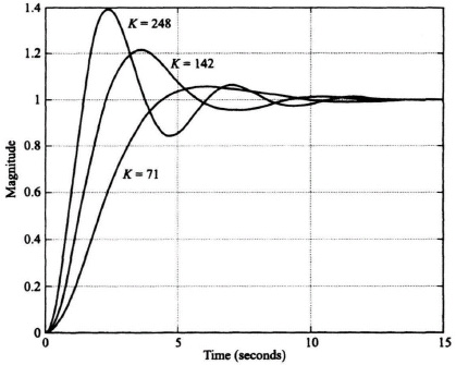
Figure 8.24 Unit step response for system of Figure 8.23 with KGc2(s)G0(s) given by Eq. (8.203) and Gc1(s) = 1.
Table 8.1. Characteristics of the Control System illustrated in Figure 8.23 where KGc2(s)G0(s) is given by Eq. (8.203), Gc1(s) = 1
| k | Damping ratio | Roots of characteristic equation |
| 248 | 0.277 | −5.1640, −20.0649, −0.3856 ± j1.3348 |
| 142 | 0.444 | −5.0878, −20.0325, −0.4398 ± j0.8875 |
| 71 | 0.666 | −5.0456, −20.01629, −0.4691 ± j0.5245 |
The design approach for this robust controller, Gc2)(s), is to place two zeros at (or near) the desired complex, conjugate-loop, poles at −0.4398 ± j0.8875 for the nominal gain case of K = 142. Therefore,
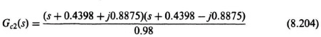
or
We will approxinate Gc2(s) as follows:
Therefore, the forward-path transfer function of this control system with KG0(s) given by Eq. (8.202) and Gc2(s) given by Eq. (8.206) is:
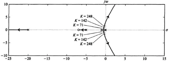
Figure 8.25 Root-locus plot for system of Figure 8.23 with KGc2(s)G0(s) given by Eq. (8.203) and Gc1(s) = 1.
Table 8.2 lists the damping ratio and the characteristic equation roots of this control system, obtained using MATLAB, with the forward-loop transfer function given by Eq. (8.207). Observe that the range of the damping ratios are much closer (0.548 to 0.808) than they were before the addition of the robust controller Gc2(s) and shown in Table 8.1 (where the damping previously varied from 0.277 to 0.666).
Figure 8.26 illustrates the root loci with the robust controller Gc2(s) added, and the location of the closed-loop, complex-conjugate, roots for the three cases. Observe from this root locus that by locating the two zeros of the forward-loop controller Gc2(s) near the desired characteristic equation complex- conjugate roots for K = 142, the sensitivity of this control system becomes much better.
It was shown in Section 8.2 during the discussion on the concept of liner-state-variable feedback that for the system illustrated in Figure 8.3, the zeros of C(s)/R(s) are the zeros of G(s) based on comparing Eqs. (8.17) and (8.24). Therefore, in the system we are currently analyzing in Figure 8.23, the zeros of the forward-path transfer function KGc2(s)G0(s) are identical to the zeros of the closed-loop transfer function. Therefore, the closed-loop zeros of Gc2(s) in Eq. (8.206) come close to canceling the effect of the complex-conjugate, closed-loop poles. Therefore, it is necessary to also add the series controller Gc1(s), as illustrated in Figure 8.23, so that Gc1(s) contains poles to cancel the zeros of s2 + 0.88 + 1 of the closed-loop transfer function. Therefore, the transfer function of the forward-loop controller, Gc1(s), is given by:
Table 8.2. Characteristics of the Control System illustrated in Figure 8.23 with the Forward-Loop Controller Gc2(s) added and where KGc2(s)G0(s) is given by Eq. (8.207).
| K | Damping ratio | Roots of characteristic equation |
| 248 | 0.548 | −6.3715, −47.3367, −0.4459 ± j0.6814 |
| 142 | 0.644 | −6.0358, −33.3566, −0.4538 ± j0.5392 |
| 71 | 0.808 | −5.6914, −26.5282, −0.4652 ± j0.3387 |
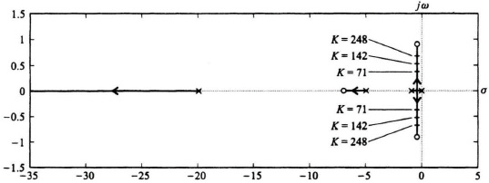
Figure 8.26 Root-locus plot for system shown in Figure 8.23 with KGc2(s)G0(s) given by Eq. (8.207).
The unit step response of this control system with the forward-path transfer function of the control system given by Eq. (8.207), with K = 71, 142, and 248, and with the forward-loop controller transfer function given by Eq. (8.208) is illustrated in Figure 8.27. Comparing these unit step responses with those in Figure 8.24, we conclude that this control system has been made to be much less sensitive to variations in K. For example, the maximum percent overshoot of the transient responses for the original system illustrated in Figure 8.24 ranged from 5.6% (for K = 71) to 39% (for K = 288). However, the control system designed to be robust has a transient response as illustrated in Figure 8.27 which shows that the maximum percent overshoot varies from 1.4% (for K = 71) to only 13% (for K = 288). In addition, as we pointed out before in comparing Eqs. (8.198) and (8.201), which are identical, the robustness with respect to variations in K will also provide disturbance suppression using the same control-system techniques.
Since the disturbance suppression attributes are a function of frequency, let us examine the frequency characteristics of the C(s)/D(s) transfer function. Substituting Eq. (8.203) into Eq. (8.198), we obtain the following transfer function for C(s)/D(s) for the case where the forward-loop controller Gc2(s) has a gain equal to one:
Substituting Eq. (8.207) into Eq. (8.198), we obtain the following transfer function for C(s)/D(s) for the case where the forward-loop controller Gc2(s) has the transfer function given by Eq. (8.206)
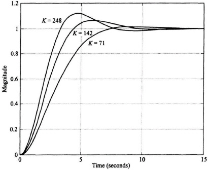
Figure 8.27 Unit step response for system of Figure 8.23 with KGc2(s)G0(s) given by Eq. (8.207) and Gc1(s) given by Eq. (8.208).
Figure 8.28 is a plot of the frequency response of the disturbance suppression transfer fucntion C(s)/D(s) as defined in Eqs. (8.209) and (8.210). It shows that the disturbance suppression of the control system at low frequencies is approximately the same with and without Gc2(s) in the control system. However, the addition of Gc2(s), as defined by Eq. (8.206), greatly improves the disturbance suppression attributes of the control system at high frequencies. This is consistent with our expectations.
Robust control-system design principles are being applied to many, modern, practical control systems. For example, the reader is referred to Reference 15 which presents the design for a robust control system for preventing car skidding. A complete case study for the design of a robust control system for controlling the flaps of a hydrofoil is presented in Section 6.7 of the accompanying volume.