PROBLEMS

8.1. The control system illustrated in Figure P8.1(i) contains linear-state-variable-feedback elements h₁ and h₂.

(a)  Determine the gain K and the linear-state-variable-feedback constants h₁ and h₂ so that the resulting control system represents a zero steady-state step error system and its characteristic equation contains roots at −2 + j, −2 − j, and −8.

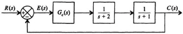
Figure P8.1(i)

(b)  The same performance can be obtained as in part (a) if we implement a series controller, G_c(s), instead of using linear-state-variable-feedback as illustrated in the configuration shown in Figure P8.1(ii).

Figure P8.1(ii)

Determine the transfer function of G_c(s) in terms of K, h₁, and h₂ obtained in part (a) and the other system parameters provided.

8.2. A control system containing a controller and a process are illustrated in the block diagram in Figure P8.2(i).

Figure P8.2(i)

(a)  Determine the state equations of this control system.

(b)  Determine the characteristic equation from knowledge of P.

(c)  Determine the constant h₁ and the gain K if the roots of the characteristic equation are at −6 and −8.

(d)  Instead of using the controller configuration, the control-system engineer wishes to design a “proportional plus integral controller” whose transfer function, G_c(s), is given by:

and is shown in figure P8.2(ii).

Determine the values of K_p and K₁ so that the roots of the characteristic equation are also at −6 and −8.

Figure P8.2(ii)

(e)  Which design would you select, the controller configuration of part (a) or the proportional plus integral controller of part (d).

8.3. The controllability and observability of the control system shown in Figure P8.3 is to be determined.

Figure P8.3

(a)  Find the state and output equations of this control system.

(b)  Determine the D matrix. Is the system controllable?

(c)  Determine the U matrix. Is the system observable?

8.4. Synthesize a system utilizing linear-state-variable feedback that has closed-loop poles existing at −9, 0 and −16, 0 and can satisfy the following specifications:

K_v = 1,    ζ = 0.707,    ω_n = 1.

It is assumed that the process to be controlled has a transfer function given by G(s) = 20/[s(s + 1)(s + 10)], and the transient response is governed by a pair of dominant complex-conjugate poles.

8.5. Repeat Problem 8.4 for the following specifications:

8.6. Repeat Problem 8.4 for the following specifications:

8.7. It is desired to synthesize a system using linear-state-variable feedback which has a closed-loop pole at −4, 0 and can satisfy the following specifications:

K_v = 1,    ζ = 0.707,    ω_n = 1.

It is assumed that the process to be controlled has a transfer function given by

and the transient response is governed by a pair of dominant complex-conjugate poles.

(a)  Can the system specifications of velocity constant be met with a simple second-order system?

(b)  What must be added to the closed-loop system transfer function?

(c)  What must be added to the open-loop system transfer function?

(d)  Synthesize the block-diagram configuration of the linear-state-variable feedback configuration for the resulting system.

(e)  Determine all unknown network constants and linear-state-variable feedback coefficients.

(f)  Draw the root locus, and determine whether the resulting synthesized system is stable. If it shows that the system is unstable, what might be done to stabilize the system?

8.8. It is desired to synthesize a system using linear-state-variable feedback which can satisfy the following specifications:

K_v = 100/sec,   yω_n = 100,    ζ = 0.5.

The process to be controlled has a transfer function given by

and assume that the transient response is governed by a pair of dominant complex-conjugate poles.

(a)  Can the system specifications be met with a simple second-order system?

(b)  Synthesize the block-diagram configuration of the linear-state-variable feedback for the resulting system.

(c)  Determine all unknown constants (if any) and all linear-state-variable feedback coefficients.

(d)  Determine whether the resulting synthesized system is stable using the root-locus method for solution.

8.9. Synthesize a system using linear-state-variable feedback that has a closed-loop transfer function given by

It is assumed that the process to be controlled has a transfer function given by

In your solution, show the following:

(a)  Synthesis of the linear-state-variable feedback system.

(b)  Identification of any compensation network needed to satisfy the synthesis.

(c)  Check of the stability of the resulting system synthesized using the root-locus method.

8.10. A control system is defined by the following:

(a)  Determine whether the system is controllable.

(b)  Determine whether the system is observable.

8.11. The state and output equations of a second-order system are given by the following:

₁(t) = –8x₁(t) + 4u(t),
₂(t) = –2x₂(t) + u(t),  
c(t) = x₁(t)               

where x₁(t) and x₂(t) represent the system state, c(t) is its output, and u(t) is its input.

(a)  Determine whether the system is controllable.

(b)  Determine whether the system is observable.

8.12. A control system is defined by the following:

(a)  Determine whether the system is controllable.

(b)  Determine whether the system is observable.

8.13. Design a second-order controller which is to be critically damped, and whose two second-order roots are located at −7 in the s-plane. The transfer function of the system to be controlled is given by

Find the vector K.

8.14. Repeat Problem 8.13 if the controller is critically damped, but its two second-order roots are now located at −4 instead of −7.

8.15. Design a second-order estimator for a system which is to have a damping ratio of 0.5, and whose estimator has two second-order roots located at −30 in the s-plane. Find the vector M. Assume that ω_n = 1 rad/sec.

8.16. Repeat Problem 8.15 if the two estimator roots are located at −15 instead of −30.

8.17. Design a second-order estimator which satisfies the ITAE criterion for a zero steady-state step error system. Assume that ω_n = 25 rad/sec.

8.18. We wish to design a regulator system (where the reference input equals zero) containing a combined controller and estimator as illustrated in Figure 8.19. The process’ transfer function is given by the following expression:

(a)  Determine the state and output equations of this process.

(b)  We wish to design the controller whose design specifications are for ω_n = 2 rad/sec and for ζ = 1. Determine the controller gain matrix, K.

(c)  We wish to design the estimator to have a much faster response than the controller. Therefore, we will design the estimator to have ω_n = 20 rad/sec and ζ = 1. Determine the estimator gain matrix M.

(d)  Determine the resulting compensator’s transfer function, U(s)/C(s).

(e)  We wish to extend the design of this sytem to the case of a system containing a reference input, r(t), as shown in Figure 8.22. Determine the vector N so that the estimator error is independent of r(t). Assume that A = 10.

8.19. Repeat the problem solved in Section 8.6 using Ackermann’s Formula for a process transfer function given by

and the control system’s signal-flow graph is shown in Figure P8.19.

Figure P8.19

(a)  Determine the state equations for the process.

(b)  Determine the controllablity matrix for this original system. Is the system controllable?

(c)  Transform the original system to the phase-variable form, and determine the state and output equations.

(d)  Determine the controllability matrix for the phase variable form.

(e)  Determine the transformation matrix A.

(f)  Design a controller assuming that the dominant pair of complex-conjugate roots has a damping ratio of 0.707, and it results in a settling time of 4 sec. Select the third pole at the location of the zero of the process to be controlled. What is the resulting characteristic equation of the desired closed-loop control system?

(g)  Determine the state and output equations for the phase-variable form with linear-state-variable feedback.

(h)  What is the resulting characteristic equation for the set of equations found in part (g)?

(i)  Determine the linear-state-variable feedback constants for the control system in phase-variable form.

(j)  Transform the linear-state-variable feedback constants back to the original system using the transformation matrix A.

(k)  Draw the resulting closed-loop control system with linear-state-variable feedback.

8.20. Determine the closed-loop transfer function of the resulting closed-loop control system developed using Ackermann’s Formula and shown in Figure 8.17, and compare it with the desired closed-loop transfer function given by Eq. (8.107). Do they agree?

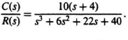
8.21. The design of the positioning system of a tracking radar is a very interesting control-system problem. Figure P8.21(a) illustrates a tracking radar which has wind torque disturbances acting on it, and the equivalent block diagram for one axis of the tracking radar’s positioning loop is illustrated in Figure P8.21(b). The block diagram illustrated represents a two-degrees-of-freedom robust control system which has the dual capability of minimizing the effects of the wind torque disturbance D(s) while also being robust (insensitive) to variations in the gain K. The transfer function for the forward-loop transfer function for the tracking radar G₀(s) is given by

(a)  Determine the transient response of this control system to a unit step input at R(s) assuming that G_c1(s) = G_c2(s) = 1 and K has a nominal value of 40, but can also vary as low as 10 and as high as 160.

(b)  Draw the root locus for the conditions in part (a). Determine the location of the closed roots for K = 10, 40, and 160, and determine the damping ratio for the dominant complex-conjugate roots for these three cases.

(c)  Design G_c2(s) so that it contains the zeros which cancel the complex-conjugate roots for the case of nominal gain 40.

Figure P8.21  A tracking radar conceptually illustrating disturbance torques due to wind forces (a), and the equivalent block diagram of the tracking radar’s positioning loop (b).

(d)  Draw the root locus for the conditions of part (c). Determine the location of the closed-loop roots for K = 10, 40, and 160, and determine the damping ratio for the dominant complex-conjugate roots for these three cases.

(e)  Design the robust controller G_c1(s), and plot the resulting transient response of this control system containing G_c1(s) and G_c2(s), which was designed in part (c).

(f)  How do the transient responses of part (e) compare to the transient responses of part (a)? Discuss the robustness of your resulting design to variations in the gain K.

8.22. The optimum sensitivity for the control system illustrated in Figure P8.22 is to be determined in the H^∞ sense. The proces G(s) has a transfer function given by

The weighting function, W(s), is given by

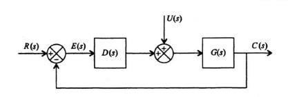
Figure P8.22

(a)  Determine B_p(s).

(b)  Determine B′(s).

(c)  Determine k.

(d)  Determine S(s).

(e)  Determine the magnitude of the optimum value of the sensitivity function, |S(jω)| as a function of T.

(f)  From your results for |S(jω)| in part (e), plot the magnitude of the optimum sensitivity function as a function of ω for T = 0.2, 2 and 20.