2.21.  STATE-VARIABLE CONCEPTS

In the analysis of a system via the state-variable approach, the system is characterized by a set of first-order differential or difference [3, 5] equations that describe its “state” variables. System analysis and design can be accomplished by solving a set of first-order equations rather than a single, higher-order equation. This approach simplifies the problem and has several advantages when utilizing a digital computer for solution. It is also the basis of optimal-control theory.

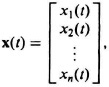
What is meant by the state of a system? Qualitatively, a system’s state refers to the initial, current, and future behavior of a system. Quantitatively, it is defined as the minimum set of variables, denoted by x₁(t₀), x₂(t₀),…,x_n(t₀) that are specified at an initial time t = t₀, which together with the given inputs u₁(t), u₂(t),…, u_m(t) for t t₀ determine the state at any future time t t₀ [4, 11–14]. We can view the state of a system, therefore, as describing the past, present, and future behavior of the system.

What is meant by the term state variables? These are the variables which define the smallest set of variables which determine the state of a system. Physically, this means that a set of state variables x₁(t₀), x₂(t₀),…, x_n(t₀) define the initial state of the system based on past history. In addition, the set of state variables x₁(t), x₂(t),…,x_n(t) characterizes the future behavior of the system once the inputs u₁(t), u₂(t),…,u_m(t) for t ≥ t₀ are specified, together with the knowledge of the initial state. It is important to emphasize that state variables are not necessarily system outputs and may not always be accessible, measurable, observable, or controllable. (Controllability and observability are discussed in Chapter 8, Sections 8.4 and 8.5, respectively.)

What is meant by the term state vector? This is a vector which completely describes a system’s dynamics in terms of its n-state variables. Therefore, given the initial state and the input u(t), a system’s state vector x(t) completely defines the system’s state for t t₀.

What is meant by the term state space? This refers to an n-dimensional space consisting of the x₁, x₂,…,x_n axes. A specific state is a point in the state space.

The motivation for using the state-variable model is to use a representation of the system dynamics that contain the system’s input-output relationship (similar to that of a transfer function) but in terms of n first-order differential equations to represent the nth order system. This approach has the following advantages:

1. The solution to a set of n first-order differential or difference equations is much easier to determine on a digital computer than the solution of the equivalent higher-order differential or difference equation. This facilitates computer-aided analysis and design on digital computers for higher-order systems. It is important to note that the Laplace transform/transfer function/block-diagram approach is inadequate for this purpose.
2. The state-variable concept greatly simplifies the mathematical notation by utilizing vector matrix notation for the set of first-order equations.
3. The inclusion of the initial conditions of a system in the analysis of control systems, which is difficult using conventional techniques, can be accounted for readily in the state-variable approach.
4. The state-variable representation lends itself to system synthesis using optimal control techniques (discussed in Chapter 6 of the accompanying volume).

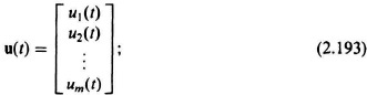
Let us consider the simple system illustrated in Figure 2.25 in order to define the nomenclature used in the state-variable approach. The system’s inputs are represented by inputs u₁(t), u₂(t),…,u_m(t), and the system’s outputs by c₁(t), c₂(t),…,c_q(t). Systems with more than one input and/or more than one output are denoted as multiple-input/multiple-output or multivariable systems. It is desirable to represent the inputs by an input vector u(t), where

the outputs are represented by an output vector c(t), where

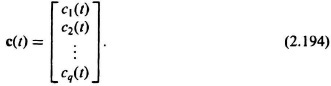
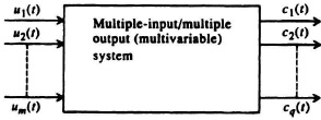
Figure 2.25   A multivariable system.

Let us next develop the general form of the state-variable equations. The system represented by Figure 2.25 has an output vector c(t) that depends on the initial value c(t₀) and the input vector u(t) for t t₀. Because the system must contain devices which remember values of the input for tt₀, we will assume that this memorization is performed by integrators, and their outputs represent the variables defining the system’s states. Therefore, we will represent the outputs of these integrators as the state variables.

For our general representation, we will assume a multiple-input and multiple-output system as shown in Figure 2.25, which has m inputs u₁(t), u₂(t), u₃(t),…,u_m(t), q outputs c₁(t), c₂(t), c₃(t),…,c_q(t), and contains n integrators. Because an nth-order system requires n states to represent it, we will represent the n-state variables to the outputs of the integrators as x₁(t), x₂(t),…,x_n(t). We will assume that we are considering initially linear, time-invariant, systems. Nonlinear and time-varying systems will be considered afterwards. Therefore, the system can be represented by the following linear n first-order differential equations, where the dot notation is used to indicate derivatives:

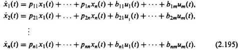
We can simplify this set of n first-order differential equations by using matrix equations:

Using the state-vector differential equation representation of Eq. (2.196), we obtain the following simpler representation of the system:

where P and B are n × n and n × m coefficient matrices, respectively, x(t) is the state vector defined by

(t) is its derivative, and u(t) is the input vector defined by Eq. (2.193). Matrix P is defined as the state or companion matrix, and B is defined as the input matrix. The solution to this vector matrix equation is uniquely determined by x(t₀) and u(t₀, T) where u(t) is defined for the interval t₀ t T. The system’s output is related to the inputs and the state variables of the system by the following vector matrix equation:

where c(t) is the output vector (q × 1) defined by Eq. (2.194), L is defined as the output matrix (q × n), and D is a coefficient matrix (q × m) which represents the direct transmission between input and output. Equation (2.197) is defined as the state equation of the system, and Eq. (2.198) is defined as the output equation of the system. Together, they are referred to as the phase-variable canonical form.

It is interesting to analyze the block-diagram representation of the phase-variable canonical form (Eqs. (2.197) and (2.198) which is shown in Figure 2.26. In most practical problems, there is no direct transmission between input and output. Therefore, D is zero in most cases, and the phase variable canonical form reduces to

For this case, the block diagram of Figure 2.26 reduces to that illustrated in Figure 2.27. It is this system and the phase-variable canonical form representation of Eqs. (2.199) and (2.200) that will be used to represent most of the systems in this book.

For simpler cases where there is only one input, the matrix B becomes a column vector, and u(t) becomes a scalar. For systems containing one input and one output, the output c(t) becomes a scalar, and the matrix L becomes a row vector.

Equations (2.199) and (2.201) are the state and output equations for linear time-invariant systems only. The state and output equations of general nonlinear and/or time-varying systems are given by

In these equations, u is an m vector, x is an n vector, and c is a q-vector.

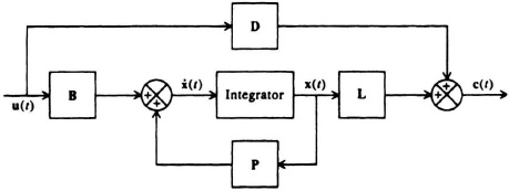
Figure 2.26   Block-diagram representation of the phase-variable canonical form.

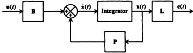
Figure 2.27   Block-diagram representation of the phase-variable canonical form without direct transmission between input and output (D = 0).

A time description of the controlled process can be obtained by solving the differential equations (2.199) or (2.201). The solution is represented as

The above equation is interpreted as the value of x(t) at time t after starting at time t₀, in state x₀, and governed by the control input u(t), defined for the interval to t₀ t T.

In the remainder of this section, several examples are given for converting the dynamics of a system (given in any of several forms) into the phase-variable canonical form.

Let us next apply this concept to several examples:

Example 1. For the first example, let us consider an open-loop system, the transfer function of which is given by

The differential equation corresponding to this system is given by

Defining the state variables as

the system can now be described by the following three first-order differential equations:

Therefore, the system can be described in the phase-variable canonical form by

where

The set of state variables selected for this problem in Eq. (2.206) is not unique for this system. Another set of state variables may be defined as long as the state vector describes the same information about the system’s behavior. Figure 2.28 shows the block diagram representation of the state and output equations from Eqs. (2.210) and (2.111), respectively. Observe that the transfer function of the feedback elements are identical to the negatives of the coefficients of the differential Eq. (2.205).

Example 2. As a second example concerned with obtaining the phase-variable canonical form of a system, consider the closed-loop system shown in Figure 2.29. The closed-loop transfer function of this system is given by

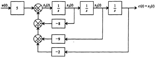
Figure 2.28   Block diagram representation of the system described by Eqs. (2.210) and (2.211).

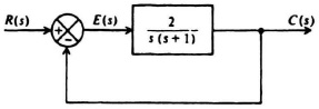
Figure 2.29   A feedback control system.

The corresponding differential equation is given by

By defining the state variables as

the system can be described by the following two first-order differential equations:

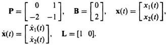
Therefore, the entire system can be described in the phase-variable canonical form by

where

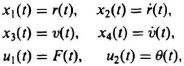
Example 3. In the third example used to illustrate the representation of the dynamics of a system in state-variable form, consider the problem of rocket flight in two dimensions. Representing the vertical and horizontal axes by v(t) and r(t), respectively, the describing equations are given by

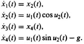
where F is thrust force per unit mass, θ is thrust direction relative to the r axis, and g is the gravitational force. The control inputs are considered to be F(t) and θ(t). Defining

we find that the dynamics are described by

This system can also be described in phase-variable canonical form by

where